By: Rohan Sikand
This is a "cheatsheet" style guide/reference to the PyTorch deep learning framework.
Part 1: Tensors
Tensors
Creating tensors from data
From data
For the following, we will use this Numpy array:
import numpy as np
data = np.array([1,2,3]) # data must be a list (convert to it if not)
Python
Four different methods:
The first two creation methods make a new copy of data in memory. Thus, changes to data will not persist.
1.
Use tensor class constructor
# floats are output no matter what
torch.Tensor(data)
Python
>>> tensor([1., 2., 3.])
The following methods are factory functions and keep the original data type for the elements.
2. Helper function of tensor class (recommended)
torch.tensor(data)
Python
tensor([1, 2, 3]) —> notice that the output's elements matches the original data type.
The following two creation methods share memory with the variable data (for efficiency). Thus, changes to data will persist in the use of these tensors.
3. Conversion
torch.as_tensor(data) # good for tuning purposes
Python
tensor([1, 2, 3])
4. Convert from Numpy
torch.from_numpy(data)
Python
tensor([1, 2, 3])
Creating tensors from no data
No data
Five different methods:
1.
Blank tensor
This can be done with any of the creation methods above (though certain data types may need to be passed as an argument).
blank_tensor = torch.tensor([]) # notice the list since this is a factory function
Python
2. Identity matrix
t = torch.eye(2) # 2 is length
Python
tensor([[1., 0.],
[0., 1.]])
3. Zeros
# rank-2 tensor (matrix) of all zeroes
torch.zeros(2,2)
Python
>>> tensor([[0., 0.],
[0., 0.]])
4. Ones
# rank-2 tensor (matrix) of all ones
torch.ones(2,2)
Python
tensor([[1., 1.],
[1., 1.]])
5. Randomly
# now randomly
torch.rand(2,2)
Python
tensor([[9.8695e-01, 2.4953e-01],
[2.9093e-04, 3.6924e-01]])
Tensor attributes
The following tensor is used for the examples t = torch.Tensor().
Data type
This attribute specifies the type of data of the elements contained within the tensor (i.e. 32-bit floating point)
t.dtype
Python
torch.float32
Full list of data types
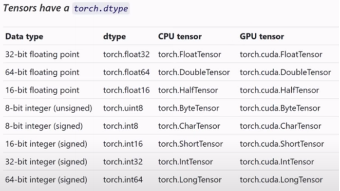
Notice that there is no strings allowed.
Changing data type
In tensor creation, you can actually override the data type and specify the one you want.
t = torch.tensor([[1,1,1,1,1]], dtype=torch.float32)
Python
Device
Find what hardware the tensor is being stored on (and all of its associated computations).
t.device
Python
cpu
Note that you will get an error if you try to perform computations between tensors stored on different devices. You will get the following error:
Error statement
>>> Expected all tensors to be on the same device, but found at least two devices, cuda:0 and cpu!
PowerShell
Layout
This tells us how the data is laid out in memory For more theory, read this.
Just know that the standard layout is strided.
t.layout
PowerShell
torch.strided
Moving tensors to a GPU
See if you are connected to a GPU
torch.cuda.is_available()
Python
Google Colab connected to GPU works!
Check version of CUDA
torch.version.cuda
Python
Moving a tensor to GPU
By default, tensors are stored on a CPU—even if you have a GPU installed. Thus, you must manually know when to convert something to be on a GPU.
# create a sample tensor
import torch
example_tensor = torch.tensor([1,2,3])
print(example_tensor)
>>> tensor([1, 2, 3])
Python
Making a tensor which will be on a CPU by default
Now convert example_tensor to utilize the GPU using CUDA:
CUDA_tensor = example_tensor.cuda() # use this command
# output
print(CUDA_tensor)
>>> tensor([1, 2, 3], device='cuda:0') # notice the device named parameter appears
Python
Failure to do this before training, even when a GPU is connected, may result in very long training time.
A note on GPU computation
Moving to the GPU is in it of itself a costly move for efficiency. Thus, it should be done not so often—only when necessary. Also, paradoxically, CPUs-especially for simple calculations-are more efficient in certain scenarios.
Thus, it is recommended that you use GPUs for training with tensors.
Rank, axis, and shape
Three very important concepts about the theoretical representation of a tensor—and they are all associated with one another.
Rank
The rank of a tensor refers to the number of dimensions in that tensor. A -dimensional tensor is considered a rank- tensor.
The number of dimensions is equivalent to how many indices we need to specify to access an individual element.
In code, to identify the rank of a tensor, take the length of its shape (for more information on shape, view below):
len(sample_tensor.shape)
Python
More conveintantly, use PyTorch's dim method:
sample_tensor.dim()
Python
Returns an int
Axis
In short, an axis of a tensor is a specific dimension of a tensor. The length of each axis, tells us how many elements are available along said axis. Note that 'dim' is another word for axis.
For example, in a 2d array, the elements of the first axis would be each row. Then, the elements of the second axis would be all of the elements in each row.
Shape
Shape is an important concept in machine learning. More often than not, a lot of errors will have to do with shape.
The shape of a tensor shows length of each axis. It is stored in an object instance of the torch.Size class which is similar to a tuple. Thus, in PyTorch .shape and .size() yield the same thing.
This is useful because once we get to higher dimensions, we won't be able to visualize some dimensions, so knowing the length of each axis (dimension) is helpful and gives us concrete information to work with.
Get the shape of a tensor
l = [
[3,4,5],
[1,2,3],
[7,6,4],
]
# convert to tensor
l_tensor = torch.tensor(l)
l.shape
Python
>>> (3, 3)
As you can see, the shape is the length along each axis.
In other words, the shape contains the how many index values (number of elements) are available along each axis.
Reshaping
Reshaping is important for neural networks, and is thus covered more in depth in its own toggle (see tensor operations). Though, it is touched on briefly here.
As tensors "flow" throughout our neural networks, different shapes are required at different points in the network. Thus, we will often need to reshape our tensors.
Thus, as programmers, we must understand the incoming shape and reshape as needed.
However, it should be noted though, that the goal fo reshaping is not to change the meaning of the data held in the tensor, but rather to shift the grouping of it.
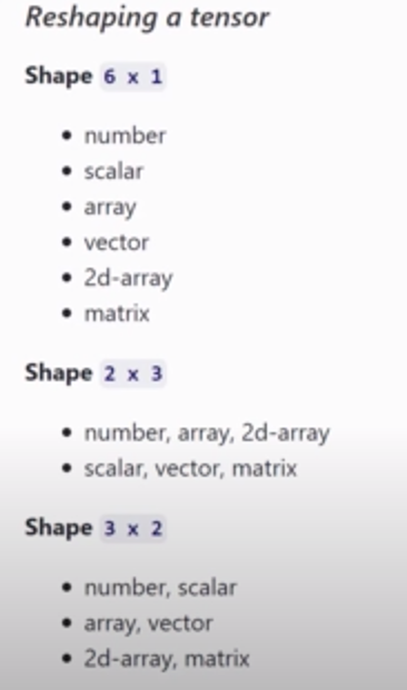
Notice that the terms are grouped differently for each specific shape, but the meaning stays the same
A note about reshaping
When reshaping, the total number of elements must be the same. In other words, the product of the numbers inside the tuple of the reshape command (i.e. a_tensor.reshape(1,9)) must be the same for the tensor you are reshaping and the resultant tensor shape.
import torch
arr = [
[3,4,5],
[1,2,3],
[7,6,4]
]
og_t = torch.tensor(arr)
print(og_t.shape)
>>> (3, 3)
print(og_t)
>>> tensor([[3, 4, 5],
>>> [1, 2, 3],
>>> [7, 6, 4]])
new_t = og_t.reshape(1, 9)
print(new_t.shape)
>>> (1, 9)
print(new_t)
>>> tensor([[3, 4, 5, 1, 2, 3, 7, 6, 4]])
Python
Same content, just stored in a different fashion. Notice that 3 * 3 = 1 * 9.
Hence, there must be a slot in the data container for each individual element.
Tensor Operations
On tensor operations
There are TONS of different tensor operations. Thus, it would be useful to categorize them for pedagogical purposes. The following are the categories:
•
Reshaping operations
•
Element-wise operations
•
Reduction operations
•
Access operations
For more, see the PyTorch docs for the torch package here.
Reshaping
The theory behind reshaping is touched in the "shape" toggle in the "Tensors" section.
In PyTorch, we can reshape a tensor by calling the .reshape() command like so:
For the length of this toggle, we will use the following tensor to start with:
data = [
[3,4,5],
[1,2,3],
[7,6,4]
]
t = torch.tensor(data)
Python
Now for the syntax:
# you can choose to change the original tensor (changes persist due to mutability)
t.reshape(1,9)
>>> tensor([[3, 4, 5, 1, 2, 3, 7, 6, 4]])
# or return it to a new variable
new_t = t.reshape(1,9)
print(new_t)
>>> tensor([[3, 4, 5, 1, 2, 3, 7, 6, 4]])
Python
More 2d reshaping examples
In this example, the following tensor is used:
t = torch.tensor([
[1.,1.,1.,1.],
[2.,2.,2.,2.],
[3.,3.,3.,3.]
])
Python
This can be reshaped in these ways:
> t.reshape([1,12])
tensor([[1., 1., 1., 1., 2., 2., 2., 2., 3., 3., 3., 3.]])
> t.reshape([2,6])
tensor([[1., 1., 1., 1., 2., 2.],
[2., 2., 3., 3., 3., 3.]])
> t.reshape([3,4])
tensor([[1., 1., 1., 1.],
[2., 2., 2., 2.],
[3., 3., 3., 3.]])
> t.reshape([4,3])
tensor([[1., 1., 1.],
[1., 2., 2.],
[2., 2., 3.],
[3., 3., 3.]])
> t.reshape(6,2)
tensor([[1., 1.],
[1., 1.],
[2., 2.],
[2., 2.],
[3., 3.],
[3., 3.]])
> t.reshape(12,1)
tensor([[1.],
[1.],
[1.],
[1.],
[2.],
[2.],
[2.],
[2.],
[3.],
[3.],
[3.],
[3.]])
Python
Recall that we can reshape a tensor in any way if the components multiply to the number of elements. We are not restricted to only two dimensions for certain tensors.
Reshaping in higher than two dimensions
Take the newly defined following tensor:
t = torch.tensor([
[1.,1.,1.,1.],
[2.,2.,2.,2.],
[3.,3.,3.,3.]
])
Python
We see that the number of elements is equal to . Thus, we may break this down like so:
t.reshape(2,3,2) # 2 * 3 * 2 = 12
Python
Instead of running code, let us intuitively understand what the output would be. First, start with the last value in the reshape argument () which represents the number of individual elements in the last axis. We know that we need elements. Thus, , which means we need sets of . Which yields us the following:
[1.,1.],[1.,1.], [2.,2.],[2.,2.],[3.,3.],[3.,3.]
Python
We now have sets of (which makes sense since the first two values in the argument multiply to ). Let us break this down even further. The second value in the reshape argument is a . This means that we now have to break our sets into . . Thus, we should now have sets of . Note that the element is now the set of (not an individual number).
[[1.,1.],[1.,1.], [2.,2.]],[[2.,2.],[3.,3.],[3.,3.]]
Python
Which yields the our resulting tensor:
>>> tensor([[[1., 1.],
[1., 1.],
[2., 2.]],
[[2., 2.],
[3., 3.],
[3., 3.]]])
Python
Here are some handwritten notes on this.
Number of components (elements) in a tensor
This is highly useful for reshaping since reshaping requires there to be the same number of elements in each tensor. There are two ways to access this.
•
Take the product of constituents of the shape of a tensor:
t = torch.tensor([1,1,1])
shape = t.shape
x = torch.tensor(shape).prod()
>>> 3
Python
Note that you must call .prod() on a torch tensor and not the shape variable. Thus, this function returns a tensor.
•
Use the built in numel() function (recommended):
t = torch.tensor([1,1,1])
t.numel()
Python
Must be called on a torch tensor. This function returns a value of type int.
Squeezing/unsqueezing
Squeezing
Squeezing a tensor removes all of the axes (dimensions) that have a length of one.
To squeeze a tensor object, use the squeeze method associated with tensor objects that comes built-in with PyTorch. Pass in the original tensor and the method will return a new tensor.
t = torch.tensor([[[[[1,2,3]]]]])
t.shape
>>> torch.Size([1, 1, 1, 1, 3])
Python
Now, to squeeze:
new_t = torch.squeeze(t)
new_t.shape
>>> torch.Size([3])
Python
Or:
another_t = t.squeeze()
another_t.shape
>>> torch.Size([3])
Python
Unsqueezing
Unsqueezing a tensor adds an axis (dimension) with a length of one.
torch.unsqueeze(input_tensor, dim) → Tensor
Python
Returns a new tensor with a dimension of size one inserted at the specified position.
dim (int) – the index at which to insert the singleton dimension
Example:
x = torch.tensor([1, 2, 3, 4])
new_x = torch.unsqueeze(x, 0)
new_x
>>> tensor([[ 1, 2, 3, 4]])
Python
Notice the extra dimension added in new_x.
For a deeper understanding, recall that the dimension is equal to the number of indices that need to be specified to get to that dimension.
For example, the call torch.unsqueeze(t, 1) would result in:
t = torch.tensor([1, 2, 3, 4])
n = torch.unsqueeze(t, 1)
n
>>> tensor([[1],
[2],
[3],
[4]])
Python
Note that you can also use named parameters for this (i.e. unsqueeze(dim=0)).
In essence, these two operations allow us to change the rank of the tensor being operated on.
Concatenation
We can combine two tensors by using the cat() function:
t1 = torch.tensor([
[1,2],
[3,4]
])
t2 = torch.tensor([
[5,6],
[7,8]
])
n = torch.cat(t1, t2)
n
>>> tensor([[1, 2],
[3, 4],
[5, 6],
[7, 8]])
Python
We can also specify the dimension:
n torch.cat((t1, t2), dim=1)
n
>>> tensor([[1, 2, 5, 6],
[3, 4, 7, 8]])
Python
Flatten
More often that not, we will need to perform an operation called "flatten" on our data points when operating on them in a neural networks. More specifically, when passing our data tensors from a convolutional layer to a fully-connected dense layer, we will need to perform a flatten operation.
A flatten operation is taking all of the scalar components of a tensor and squashing them into one giant tensor of one dimension.
Thus, if we had a 2d-tensor (matrix), the flatten operation takes all of the rows and appends them to the first row to create one dimension.
Let us look at multiple ways we can achieve this:
# first solution
def flatten(t):
t = t.reshape(1, t.numel())
t = torch.squeeze(t)
return t
# second solution
t = t.reshape(-1)
# third solution
t = t.reshape(t.numel())
# fourth solution
def flatten(t):
t = t.reshape(1, -1)
t = torch.squeeze(t)
return t
# fifth solution
t = t.flatten()
Python
Negative dimension specified
If you specify a in the reshape argument, PyTorch conveniently calculates the correct value for you based on the number of elements in the tensor and the other values specified in the reshape argument. Mathematically:
Selective flattening
Motivation: theory behind CNN tensors
In convolutional neural networks, the data must be flattened when passing the tensors from convolutional layers to fully-connected layers. Also, we will be passing in batches of data points into the neural networks, so we will need to know how to flatten individual dimensions of a tensor.
Typically, this is the shape that is being dealt with for tensors that are fed into CNNS:
For example, take three sample tensors of rank-2 which could be representative of singular images.
# these are sample three images
t1 = torch.tensor([
[1,1,1,1],
[1,1,1,1],
[1,1,1,1],
[1,1,1,1]
])
t2 = torch.tensor([
[2,2,2,2],
[2,2,2,2],
[2,2,2,2],
[2,2,2,2]
])
t3 = torch.tensor([
[3,3,3,3],
[3,3,3,3],
[3,3,3,3],
[3,3,3,3]
])
Python
Creating a batch tensor
Let us now convert them into a batch. To do this, we can use the stack function:
batch = torch.stack((t1,t2,t3))
batch.shape
>>> torch.Size([3, 4, 4])
Python
Adding a color channel
For CNNs, the tensor needs to include a color channels dimension. For grayscale, this would be one, and for RGB, this would be color. As specified above, this color channel axis should be the second axis. Thus, we can simply implement a reshape command
new_t = batch.reshape(3,1,4,4)
new_t.shape
>>> torch.Size([3, 1, 4, 4])
Python
An example batch tensor which contains three images, one color channel (usually grayscale), and the height and width of each image.
Visualizing the tensor
batch_tensor = torch.tensor([ # batch of 3 images
[ # image one
[ # color channel one
[1, 1, 1, 1],
[1, 1, 1, 1],
[1, 1, 1, 1],
[1, 1, 1, 1]
],
[ # color channel two
[1, 1, 1, 1],
[1, 1, 1, 1],
[1, 1, 1, 1],
[1, 1, 1, 1]
],
[ # color channel three
[1, 1, 1, 1],
[1, 1, 1, 1],
[1, 1, 1, 1],
[1, 1, 1, 1]
]
],
[ # image two
[ # color channel one
[2, 2, 2, 2],
[2, 2, 2, 2],
[2, 2, 2, 2],
[2, 2, 2, 2]
],
[ # color channel two
[2, 2, 2, 2],
[2, 2, 2, 2],
[2, 2, 2, 2],
[2, 2, 2, 2]
],
[ # color channel three
[2, 2, 2, 2],
[2, 2, 2, 2],
[2, 2, 2, 2],
[2, 2, 2, 2]
]
],
[ # image three
[ # color channel one
[3, 3, 3, 3],
[3, 3, 3, 3],
[3, 3, 3, 3],
[3, 3, 3, 3]
],
[ # color channel two
[3, 3, 3, 3],
[3, 3, 3, 3],
[3, 3, 3, 3],
[3, 3, 3, 3]
],
[ # color channel three
[3, 3, 3, 3],
[3, 3, 3, 3],
[3, 3, 3, 3],
[3, 3, 3, 3]
]
]
])
Python
Flatten along a specific dimension
We need to flatten the image tensors before passing them into a fully-connected layer in a neural network. But we do not want to flatten everything (the whole batch) at once.
Thus, to perform flattening along a single axis, use this:
flattened_batch = batch_tensor.flatten(start_dim=1)
Python
Element-wise operations and broadcasting
Definition and correspondence
"An element-wise operation is an operation between two tensors that operates on corresponding elements within the respective tensors."
An element of one tensor is said to be corresponding to another element in another tensor if, to access said elements, the same indexes are specified.
Take the following two tensors. Each element in t1 is of the same color in the corresponding element of that element in t2.
t1 = torch.tensor([
[1,2],
[3,4]
])
t2 = torch.tensor([
[9,8],
[7,6]
])
Python
Thus:
# t1(element) corresponds to --> t2(element)
t1[0][0] = 1 --> t2[0][0] = 9
t1[0][1] = 2 --> t2[0][1] = 8
t1[1][0] = 3 --> t2[1][0] = 7
t1[1][1] = 4 --> t2[1][1] = 6
Python
Notice that the indices specified are the same for corresponding elements
Also, note that two tensors need to have the same number of elements and have to have the same shape to perform element-wise operations between them.
Why is this needed?
When a tensor is fed through an neural network, linear algebra comes into play. All of those matrix multiplications are done element-wise. It is neat to see the mathematical theory developed in code.
t1 = torch.tensor([
[1,2],
[3,4]
])
t2 = torch.tensor([
[9,8],
[7,6]
])
# element-wise operation
t3 = t1 + t2
t3
>>> tensor([[10, 10],
>>> [10, 10]])
Python
Other arithmetic operations are also element-wise operations.
Arithmetic operations using scalar values
new_t = t1 * 2
new_t
>>> tensor([[2, 4],
>>> [6, 8]])
Python
But wait... in the definition above, we specified that the two tensors must be of the same shape and size. Technically, a scalar is a rank-0 tensor... so why does this work. Let us introduce the concept of broadcasting.
Broadcasting
Broadcasting
Tensor broadcasting explains how tensors of different shapes are treated during element-wise operations.
For example, in this code,
new_t = t1 * 2
new_t
>>> tensor([[2, 4],
>>> [6, 8]])
Python
the 2 is being "broadcasted" to the shape of t1.
In PyTorch, this is done implicitly. However, let us see how this works explicitly.
import numpy as np
b = np.broadcast_to(2, t1.shape)
b
>>> array([[2, 2],
>>> [2, 2]])
Python
Now the element-wise operation is performed.
Broadcasting is often used in preprocessing and normalizing data.
Comparison operations
Comparison operations
In comparison operations, a new tensor of the same shape is returned with each element containing either a boolean value of either True or False.
l1 = torch.tensor([2,3])
l2 = torch.tensor([4,1])
l3 = l1 < l2
l3
>>> tensor([ True, False])
Python
There are also methods for comparison operators. Here is an example:
t = torch.tensor([
[0,5,0],
[6,0,7],
[0,8,0]
], dtype=torch.float32)
# >=
t.ge(0)
>>> tensor([[True, True, True],
>>> [True, True, True],
>>> [True, True, True]])
# >
> t.gt(0)
>>> tensor([[False, True, False],
>>> [True, False, True],
>>> [False, True, False]])
Python
This code snippet was taken directly from ^1 (see references below).
Methods that use element-wise operations
Methods that use element-wise operations
Some functions of tensor objects also use broadcasting (implicitly) to perform element-wise operations. Here are some examples:
# absolute value
m = torch.tensor([[-1,-2],[1,2]]
m.abs()
>>> tensor([[1, 2],
>>> [1, 2]])
# for sqrt, the dtype cannot be int (long)
m = torch.tensor([[10,22], [1,2]], dtype=torch.float32)
m.sqrt()
>>> tensor([[3.1623, 4.6904],
>>> [1.0000, 1.4142]])
Python
There are many more operations that can be performed through tensor object methods, but these are a few examples.
Also note that element-wise is sometimes referred to as "component-wise" or "point-wise".
Reduction operations (ArgMax)
A reduction operation on a tensor is an operation that reduces the number of elements contained within the tensor. More specifically, it is an operation within the scalar components of the a tensor.
Here are some examples:
t = torch.tensor([[1,2,3], [14,15,16], [17,18,19]])
s = t.sum()
s
>>> tensor(105)
type(s)
>>> torch.Tensor
Python
As you can see, a reduction operation returns a tensor.
Here are some more examples:
t.prod()
>>> tensor(117210240)
f = torch.tensor(t, dtype=torch.float32) # only works with floating point numbers
f.mean()
>>> tensor(11.6667)
Python
Specified dimension
There can also be reductions that don't result in rank-0 scalar valued tensors. For example, we can specify the dimension and utilize broadcasting.
t = torch.tensor([
[1,1,1,1],
[2,2,2,2],
[3,3,3,3]
], dtype=torch.float32)
t.sum(dim=0)
>>> tensor([6., 6., 6., 6.])
# this is done by broadcasting: t[0] + t[1] + t[2]
Python
Taken from ^1 (see references below)
t.sum(dim=1)
>>> tensor([ 4., 8., 12.])
# this is implicity doing: t[0].sum() + t[1].sum() + t2.sum()
Python
ArgMax
ArgMax is a very common operation used a lot specifically in classification outputting.
Argmax returns the index location of the maximum value inside a tensor.
t = torch.tensor([[1,2,3], [14,15,16], [17,18,19]])
t.max()
>>> tensor(19)
# to get the index, use ArgMax
t.argmax()
>>> tensor(8)
Python
Implicitly, the tensor is flattened, then the index is found. Thus, the argmax() function is operating on t.flatten() which equals tensor([ 1, 2, 3, 14, 15, 16, 17, 18, 19]).
ArgMax on a specific dimension
t.argmax(dim=0)
>>> tensor([2, 2, 2])
Python
Runs along the first axis
n = torch.tensor([[3,4], [4,5], [5,4]])
n.argmax(dim=0)
>>> tensor([2, 1])
n.argmax(dim=1)
>>> tensor([1, 1, 0])
Python
Second example runs along each array
Access operations
In Python lists, we can access an individual element with list_name[0]. But we cannot do that with tensors and have it return a data type that is usable universally with other python syntax. We can do tensor_name[0] but that still returns a tensor (type(tensor_name[0]) >>> torch.Tensor). Thus, we can use the following (and more—check out the PyTorch documentation):
tensor_example = torch.tensor([5,23,4])
tensor_num = tensor_example[2].item()
>>> 4
type(tensor_num)
>>> int
Python
Or we can just convert it into a list:
tensor_example.tolist()
>>> [5, 23, 4] (type: list)
# another example (with two dimensions)
another_tensor = torch.tensor([[4,3,34], [34,54,24]])
another_tensor[1].tolist()
>>> [34, 54, 24] (type: list)
Python
Part 2: Neural Networks and Deep Learning
A note regarding the next sections
In the next sections, we will be explaining concepts regarding an entire machine learning project. Specifically, the project is to classify fashion item images from the FashionMNIST dataset.
Data and Data Preprocessing
Extract, Transform, and Load (ETL)
To prepare data for DL algorithms, we first need to extract the data for the data source, transform that data into a desirable format, and then we can load the data into a suitable format. This pipeline is referred to as Extract, Transform, and Load (ETL).
Fortunately, PyTorch has a substantial amount built-in packages and classes that ease the ETL process.
For the project we are following along, the following pipeline for ETL is:
•
Extract - get the Fashion-MNIST image data from the official source.
•
Transform - put the data into tensor form
•
Load - put the data into an object for easy accessibility (to be fed into a DL algorithm)
Dataset
Dataset is an abstract, extendable class in PyTorch for simple data loading. When you want to write a custom dataset, you will need to write a new subclass, which inherits the Dataset abstract class.
When writing the subclass of Dataset, we will be performing the "extract" (retrieve data from source) and "transform" (convert to tensors) phases of the ETL pipeline.
Definition from the official documentation
"An abstract class representing a Dataset.
All datasets that represent a map from keys to data samples should subclass it. All subclasses should overwrite __getitem__(), supporting fetching a data sample for a given key. Subclasses could also optionally overwrite __len__(), which is expected to return the size of the dataset by many Sampler implementations and the default options of DataLoader."
What exactly is a dataset in PyTorch?
Recall that an abstract class is a class that is not meant to be initialized (i.e. cannot create an object instance it), but rather to have methods that are to be implemented. Thus, we do not actually create objects of PyTorch's Dataset class itself, but rather create a subclass that inherits from it. Then, we create an object instance of that class to obtain a dataset.
When we create an instance of our own subclass of Dataset, that is a new type of object. Daniel Godoy put it best:
"You can think of it as a kind of a Python list of tuples, each tuple corresponding to one point (features, label)." - Daniel Godoy
Dissecting this further, the dataset object that we obtain is essentially a Python list which contains tuples where the first element of each tuple is the data point and the second element is the corresponding label.
Example:
print(train_dataset[0])
>>> (tensor[[10],[20],[30]], 'nine')
print(type(train_dataset[0))
>>< tuple
Python
In this case, we have a data point in the form of a tensor and a label of 'nine'.
Writing the subclass of Dataset
For custom datasets, our job is to write the class in such a way that the object instance of the class is that list of tuples like explained above. To do this:
When when subclassing and inheriting from Dataset, we implement two of its methods.
__getitem__
This method is required to be implemented.
We should write this function such that when an index regarding dataset is given as an argument, it returns the corresponding data point tuple at that index (in conclusion, this returns a single sample from the dataset).
def __getitem__(self, index):
"""insert code here"""
pass
Python
Should return a tuple.
__len__
Gets the length of the dataset.
This method is optional to implement (though, you should do it anyway).
The reason why this is important is that when working with Dataloader, if you want to divide the dataset into batches, then you will need the length for sampling purposes (read about sampling here).
def __len__(self):
pass
# return length of dataset
Python
Furthermore, since this is a class, we need to implement a constructor. The goal here is to extract the data, transform into tensor form, and split the samples from the labels (self.X and self.y respectively). See the "full example" below which displays this.
TensorDataset
Alternatively, if our data is already in tensor format, we can wrap them using TensorDataset to generate our dataset object.
ImageFolder
Similar to Keras, PyTorch Vision (sits atop Torch) conveniently offers a prebuilt dataset class if the images are arranged like so:
root/dog/xxx.png
root/dog/xxy.png
root/dog/xxz.png
root/cat/123.png
root/cat/nsdf3.png
root/cat/asd932_.png
Plain Text
•
Can specify transformations (i.e. for data augmentation).
•
Required to specify root folder (use '.' if you are writing your code in the same folder).
An example:
train_set = torchvision.datasets.ImageFolder("data/train", transform = transformations_here)
validation_set = torchvision.datasets.ImageFolder.("data/validation", transform = transformations_here)
Python
See docs for more.
A notebook showing the concepts executed in Python.
Constructing Neural Networks
Background, overview, and motivation
In PyTorch, neural networks are constructed by layers in an object-oriented fashion. That is, each layer in the defined neural network will be an object instance of a layer class. Inside that layer class, two types of abstractions need to be written: transformation and learnable weights (and biases). Recall that writing classes consists of two things: instance variables and methods. The transformations will be defined as methods whereas the instance variables are used for the learnable weights.
Fortunately, PyTorch provides a highly-functional nn module which lets us use their predefined layers—which are objects of their respective classes. Custom layers, if need be, can also be created.
In addition to layers, we also represent entire networks as objects as well (a function of functions essentially).
Thus, we should extend PyTorch's module base class anytime we create a layer or network.
In building a layer/network, we first construct it, then create a forward method describing the transformation of the tensor inputs through the constructed network/layer.
The three steps in building neural networks with PyTorch
From :
1.
Extend the nn.Module base class.
2.
Define layers as class attributes.
3.
Implement the forward() method.
Inheriting nn.Module
When constructing a network or layer, to use PyTorch's features, inherit from the nn.Module class (line 1). Furthermore, inherit the super constructor from nn.Module (line 3) as well like so:
class Network(nn.Module): # line 1
def __init__(self):
super().__init__() # line 3
Python
"Hello, world!" neural network in Pytorch
class Network(nn.Module): # line 1
def __init__(self):
super().__init__() # line 3
self.layer = InsertLayerHere
def forward(self, t):
t = self.layer(t)
return t
Python
Simply a basic one layer dummy network.
Hyperparameters and data-dependent hyperparameters
These are the two types of parameters we will be using when constructing the layers. A parameter is a place-holder that will eventually hold (data-dependent hyperparameter) or have a value (standard hyperparameter).
The difference between the two is that standard hyperparameters do not depend on the data we are trying to process with the layer. That is, no matter what the data is, these can be the same. In contrast, data-dependent hyperparameters are parameters whose values are dependent on data. That is, the values selected for them will depend on our input data.
We, humans, set the values for these hyperparameters (not to get confused with learnable parameters). Generally, the values are chosen by fine-tuning during experimentation or by previous research that suggests certain values.
The following tables show standard and data-dependent hyperparameters for convolutional and fully-connected layers.
Standard hyperparameters
Data-dependent hyperparameters
•
in_features depends on the input data if it is the first layer. If not, then the parameter value is equal to the output of the previous layer.
•
in_channels the same applies as above if this isn't the first layer. Except, if this is the first layer, then this represents the number of color channels the image has (RGB = 3 and grayscale = 1).
•
The last layer is always a fully-connected layer in which the out_features depends on the number of classes for classification. For regression, that number depends on the number of values you are trying to predict.
Building a fully-connected linear layer
These are the most simplest layers involved in neural networks. To build one in PyTorch, we need to specify two parameters in the network's constructor: in_features and out_features. "When we construct a layer, we pass values for each parameter to the layer’s constructor".
self.fc1 = nn.Linear(in_features=60, out_features=10)
Python
60 and 10 are the arguments
If the out_features layer is the last layer:
In the network as a whole, "we shrink our out_features as we filter down to our number of output classes.".
Learnable parameters
"These are the parameters whose values are learned through the learning process"—this is where the intelligence comes from. These learnable parameters are the weights inside our network, and they live inside each layer.
Definition from deeplizard
Learnable parameters are parameters whose values are learned during the training process.
With learnable parameters, we typically start out with a set of arbitrary values, and these values then get updated in an iterative fashion as the network learns.
In fact, when we say that a network is learning, we specifically mean that the network is learning the appropriate values for the learnable parameters. Appropriate values are values that minimize the loss function.
Accessing learnable parameters
Since the layers inside the network are objects themselves, we can access their attributes (instance variables) just like any other object in Python by using dot notation. torch.nn layer objects store the learnable parameters as attributes. Thus, if we want to access the weight tensor of a particular layer of a particular network, that can be done like so:
NeuralNetwork.conv1.weight
Python
The resultant is a torch tensor.
Once data is fed into the network, these weight values inside the weight tensors are optimized—this gives us the intelligence produced by the resultant network.
String representation of NNs
String representations are what shows up when you try to print out an object,
When we build a neural network from torch.nn, we also inherit the string representation which formats the network's constituents nicely. To see this for yourself, print the object instance out.
If desired, we can override this by using __repr__:
def __repr__(self):
return "some object" # return string representation here
Python
Convolutional Neural Networks
Building a convolutional layer
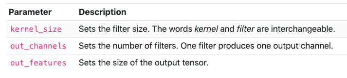
When building a convolutional layer, we need to specify three parameters: in_channels, out_channels, and kernel_size.
•
For the first layer, in_channels is determined by the number of color channels of the input data. Then there after, in_channels is simply the output of the previous layer.
•
out_channels is the number of feature maps outputted after the kernel convolves over the data.
•
kernel_size is the size of the window of the convolution operator. Interestingly, the argument is actually a tuple. If you specify one number, then a square kernel will be used.
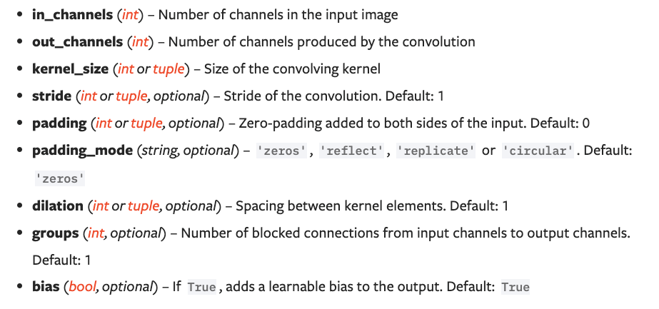
Other parameters (optional)
Here is a complete list of parameters for Conv2d layers taken from PyTorch's documentation:
We define our layer inside the constructor, as an instance variable, of our network (just like with fully-connected layers.
self.conv1 = nn.Conv2d(in_channels = 1, out_channels = 6, kernel_size = 5)
Python
A note on the layers of a convolutional neural network
Generally, we aim to increase the out_channels as we add more convolutional layers. Then, after we are done with the convolutional part of the network, we must end with a fully-connected perceptron-type layer. Though, we usually use three-four fully-connected layers to output.
Once we transition from convolutional to fully-connected, several key things occur:
•
out_features exist as the output instead of out_channels. These represent the nodes of the typical neural network architecture. Generally, in contrast to convolutional layers, we aim to start high for out_features and eventually dwindle our way down to how many classes we have (if regression, modify to number of values you are trying to predict).
•
The first in_features parameter value after all of the convolutional layers will need to be delicately determined based on the input data (a flattening process). See below for more.
References
deeplizard
This reference guide was created while watching and reading this course from the deeplizard YouTube channel. Often times, the code syntax and definitions for certain concepts just make most sense with how they defined it. Thus, for exact copy-paste situations, I indicated that that was the case through attaching a '' next to it. As mentioned below, this document is still a very rough draft version so there is a good chance that I have missed certain spots where there should be. a citation—as I update this document, I will try to manage this as best as possible.
Also please note that this document is a draft version and the sole intention of this document was to help me better understand the PyTorch deep learning framework.