Berkeley CS 182, Lecture 21 - Meta Learning

Introduction (and black-box meta-learning)

• meta learning is a new concept in machine learning that allows a general representation of a model to adapt to new tasks very quickly.
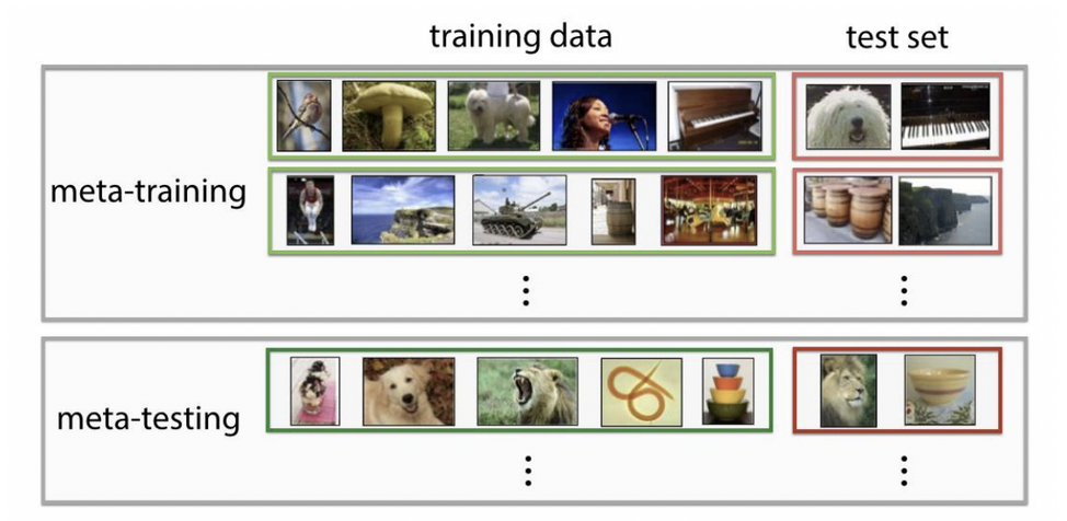
• The main idea behind meta learning is to learn how to learn. And what we mean by this is that we can represent tasks that are fundamentally different as our training samples in a large dataset, so for example, we might have a cats versus dogs task and also a hot dog versus burger classification task. But if you think about this deeply, you understand that a human who is able to learn how to classify cats versus dogs might be able to use that general representation and some of that to also classify hotdogs vs. burgers, it’ll be able to adapt to the hotdogs and burgers example much quicker than if it had not seen the cats versus dogs example in the first place and this is important because a lot of tasks in the world share general representations that underly the actual task. But most of these tasks do not have a lot of data. So the idea is that we have a lot of images of cats and dogs but little bit of burgers and hotdogs. We can learn the general representation that underlies the task of classifying images and apply it to new datasets that are smaller.
• We will cover three different meta-learning paradigms, but first let’s introduce the high-level concept (explained through the first paradigm: black-box meta-learning).
• In traditional SL, we have:

\[ f(x) \rightarrow y \]

where \(x\) is, for example, an image and \(y\) is a classification label. But in meta-learning, we have

\[ f\left(\mathcal{D}^{\operatorname{tr}}, x\right) \rightarrow y \]

where \(\mathcal{D}^{\operatorname{tr}}\) is a training dataset for some task \(T_i\), where the entire dataset for \(f\) is composed of tasks \(T_1, \ldots, T_n\).

💡 Underlying question: how do we read in a task training set into some neural network?

• For traditional SL, we’d, for example, flatten the image pixels into one long sequence and pass this into the model (i.e., an MLP).
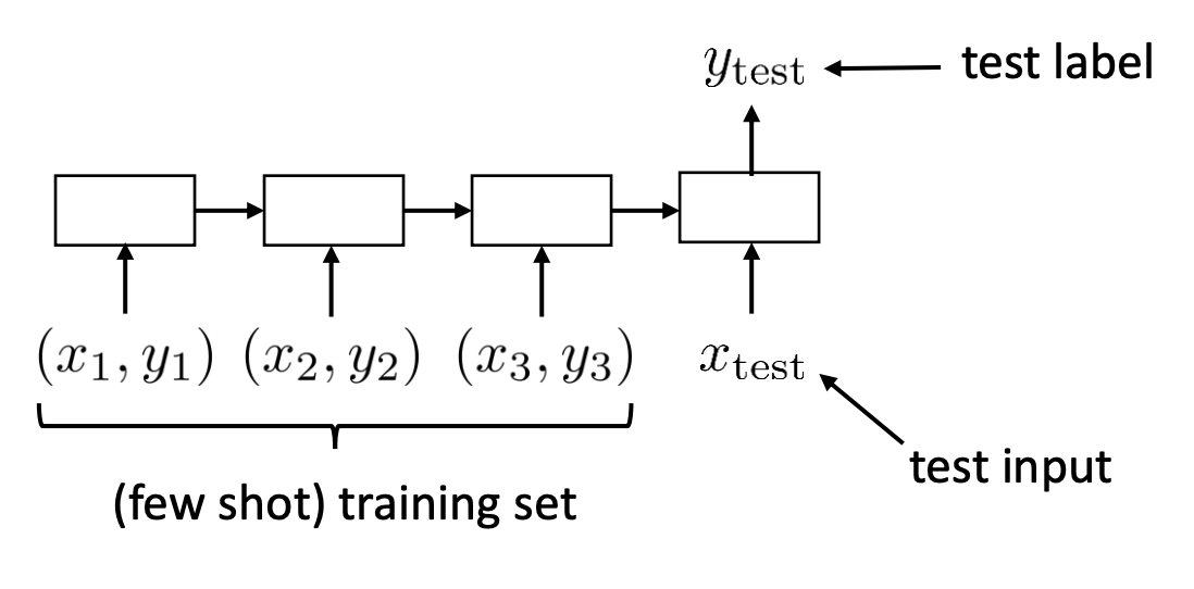
• So we can do the same here: concatenate and flatten the entire training set as a sequence and use some sequence-based model like an LSTM.
  • Note: we’d concatenate the labels to the model (one-hot vector represented) as well.
    • Zero-out the query labels though.
• Visually, we’d pass in this entire sequence for each \(\mathcal{D}^{\operatorname{tr}}\):

Generic learning vs. generic meta-learning

The following describes the same concept, just in two different perspectives. Above, we thought of this whole task as a traditional supervised learning problem where the inputs themselves are just tasks in the form of \(f\left(\mathcal{D}^{\operatorname{tr}}, x\right) \rightarrow y\). That is,

• “Generic” supervised learning (in the context of meta-learning): From here, the training process is the same as with traditional supervised learning. Just train \(f\left(\mathcal{D}^{\operatorname{tr}}, x\right) \rightarrow y\)!

However, we can also view this entire process in a different light, which we call “Generic meta-learning”.

Here is a box containing the mathematical representation of the two points.

Generic learning: \[\begin{aligned} \theta^{\star} &=\arg \min _\theta \mathcal{L}\left(\theta, \mathcal{D}^{\operatorname{tr}}\right) \\ &=f_{\text {learn }}\left(\mathcal{D}^{\operatorname{tr}}\right) \end{aligned}\]

Generic meta-learning: \[ \theta^{\star}=\arg \min _\theta \sum_{i=1}^n \mathcal{L}\left(\phi_i, \mathcal{D}_i^{\mathrm{ts}}\right) \] where \(\phi_i=f_\theta\left(\mathcal{D}_i^{\mathrm{tr}}\right)\).

Visually,

Let’s break the second view down further.

• Flatten entire task into one long sequence composed of \(\mathcal{D}^{\mathrm{tr}}_i = [(x_1, y_1),...(x_n, y_n)]\).
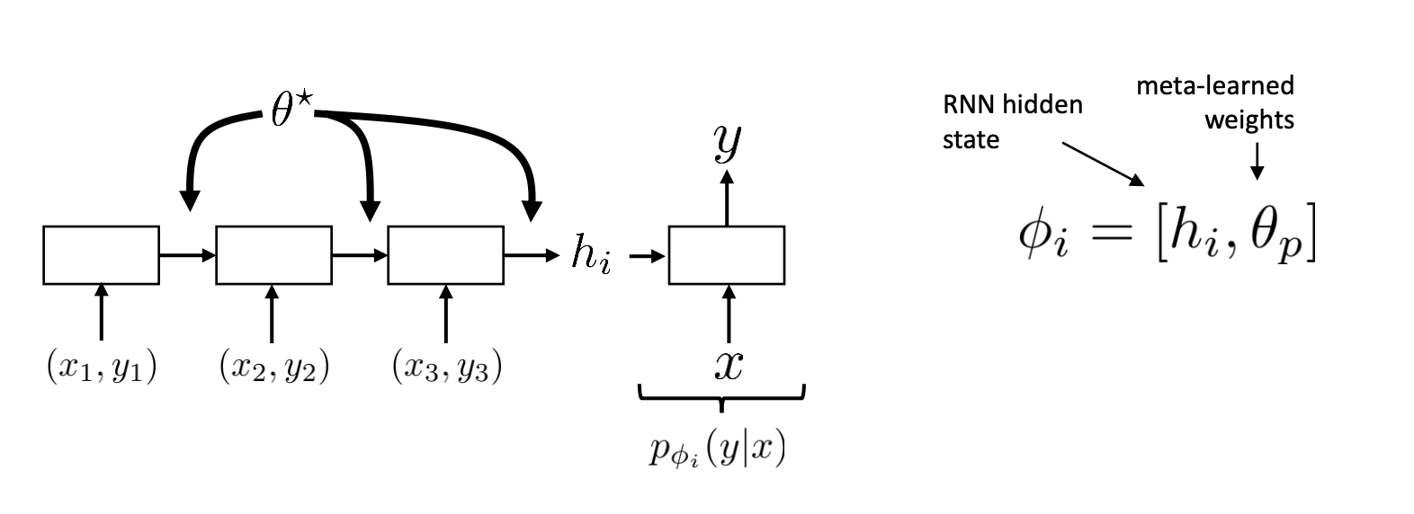
• Input this into some sequence model (i.e., an RNN). The RNN is notated as \(f_\theta\) with parameters \(\theta^{\star}\).
  • You can think of the RNN as a learnable feature extractor.
• This RNN produces the last hidden state \(h_i\). \(h_i\) contains the updates for \(p_{\phi_i}(y \mid x)\), which is a task-specific head (e.g., MLP classifier).
• So we have \(\phi_i=f_\theta\left(\mathcal{D}_i^{\mathrm{tr}}\right)\) and \(\phi_i=\left[h_i, \theta_p\right]\). Essentially, the RNN updates the classifier head’s parameters (which are separate from the overall RNN model parameters). We explicitly train to update the RNN model parameters, but implicity this meta-learns the MLP head (\(p_{\phi_i}(y \mid x)\)) parameters as well!

In practice, we’d set this up very mechanicalistically: just a sequence + label problem. Just to re-iterate:

• We pass in a flattened sequence of \(\mathcal{D}^{\mathrm{tr}}_i\), concatenated with the unlabeled test points (all of them). The desired output is the labels for those test points.

Meta-learning methods

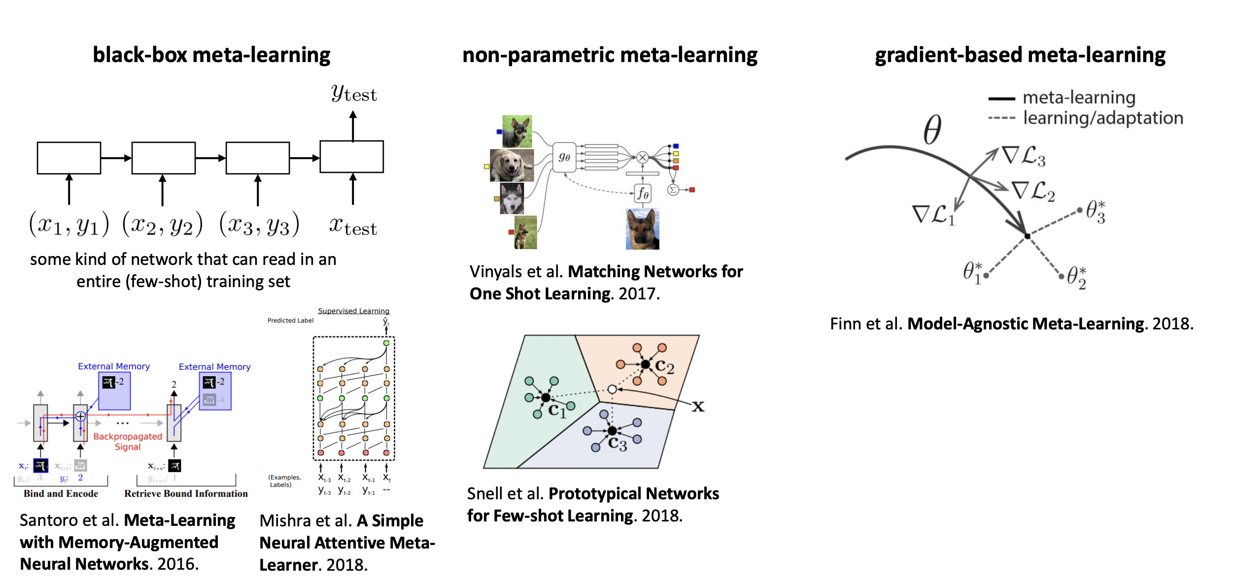
Can group them into the following three-categories:

1. Black-box meta-learning
   • recasting the meta-learning problem as a meta supervised learning problem. What we just described in the above section.
   • Generally done via sequence-based NN’s that read in \(\mathcal{D}^{\mathrm{tr}}\) entirely.
   • CS 330, hw 1
   • Note that the entire training set for a task can get very large, very quickly (\(n * k\)). Thus, advanced sequence models have been developed for this. For example, “Meta-Learning with Memory-Augmented Neural Networks” (MANN), which uses external memory to keep the entire dataset in-place. Again, what we implemented in hw 1.
   • Think of it this way: optimization process is the same, but the (meta)-model is different. Can we reverse this?
2. Non-parametric meta-learning
   • Parametric in the meta aspect, but not parametric on a per-task basis.
   • “k-means for tasks”
   • Protonets
3. Gradient-based meta learning
   • MAML
   • Adapt to new task by fine-tuning your model with gradient descent. Train in such a way that optimizes the adaptation process. Learning how to learn.
   • Optimization process is different, but the model is same (hence, “model-agnostic”).
   • This is the important one that is used more commonly nowadays.

Note

Non-parametric meta-learning

• Note that by non-parametric, we mean we don’t use params to adapt to each new task. But the overall deep net still has params.

High-level idea

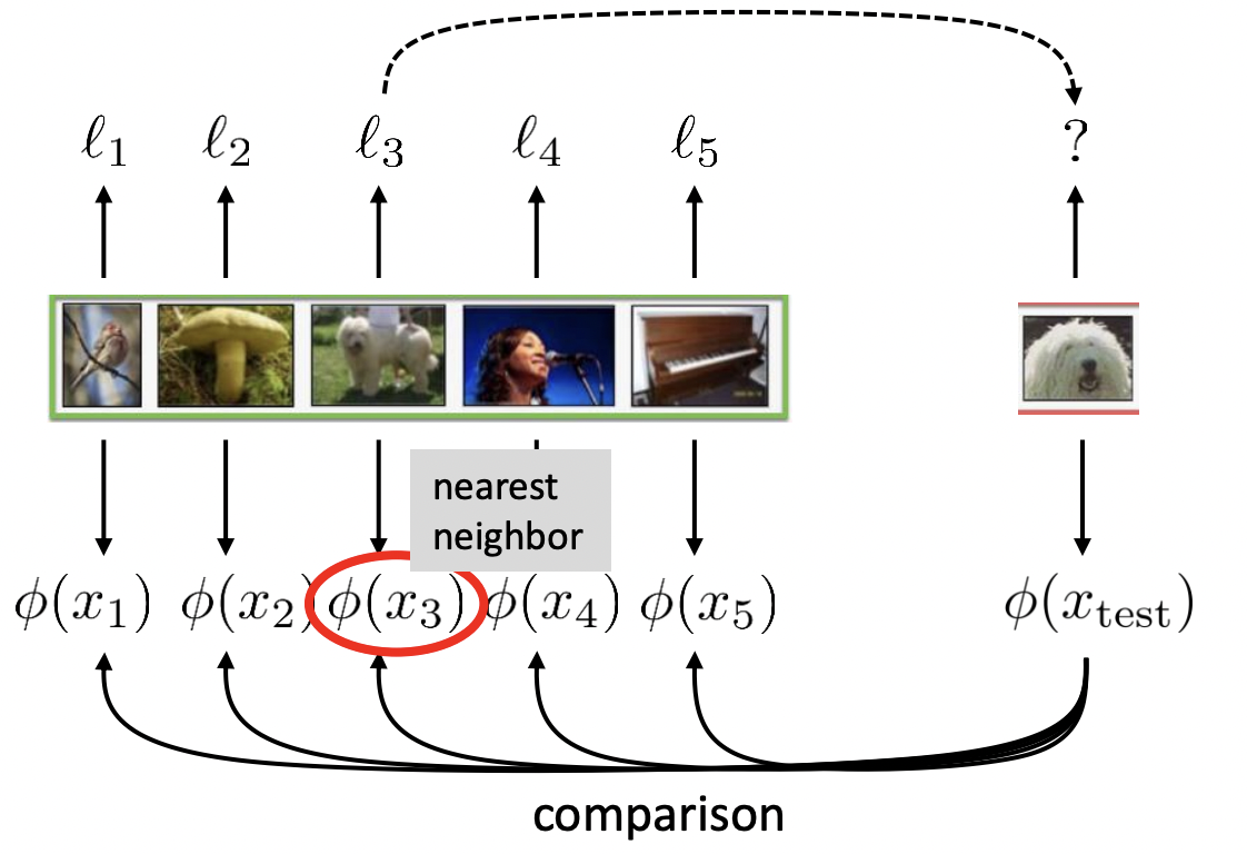
• Suppose we have a 1-shot, 5-way classification problem. We have 5 images in each \(\mathcal{D}^{\mathrm{tr}}_i\), each corresponding to a different class. We now have one new image in \(\mathcal{D}^{\mathrm{te}}_i\). We wish to assign one of the 5 labels to this new image. The idea is to compare this test image to the train images and take the label of the nearest neighbor (from the train images) to the test image.
• But the pixel values aren’t that comparable/learnable. So to make this learnable, we use an extractor network \(\phi\) to embed each images into some feature space. Then, in this feature space, we can find this nearest neighbor. But the idea is that we parameterize \(\phi\left(x_i\right)\) and learn these params during the training process.
  • The idea is to learn a good feature space.
  • Note that for now, the feature space is the same for the train and test images but they can be separate (discuss this later).
• Lots of math details, but see the video for that.

Here is the loss:

\[ \theta^{\star}=\arg \min _\theta \sum_{i=1}^n \mathcal{L}({f_\theta\left(\mathcal{D}_i^{\mathrm{tr}}\right.}), \mathcal{D}_i^{\mathrm{ts}}) = -\sum_{i=1}^n \sum_{j=1}^m \log p_\theta\left(y_j^{\mathrm{ts}} \mid x_j^{\mathrm{ts}}, \mathcal{D}_i^{\mathrm{tr}}\right) \]

where the parameters \(\theta^{\star}\) are learned for the embedding network/function \(\phi(x)\).

Ok… we got the high-level idea down. Now let us turn to some actual implementations (which are a bit more involved).

Matching networks

…

Optimization-based Meta Learning

We will cover MAML. There also exists Reptile which avoids second derivatives.

• We can model the inner loop optimization process as a “model” that we, in it of itself, optimize.
• Idea is to run gradient descent quickly for fast adaption to new tasks.
• Inner loop: adaptation to new task
• The general idea is to have two notions of the parameters for a model:
  • \(\theta\) as the “meta” parameters.
  • \(\phi_i\) as the task-specific parameters of the model learned for \(T_i\).
• The idea is to optimize \(\theta\) overall such that a few gradient steps for each task will result in good \(\phi_i\) parameters.

MAML pseudocode:

0. randomly init theta
1. Sample task from dataset 
    a. extract support and query 
2. update phi_i through a few gradient descent steps
3. update meta parameter theta by computing gradient of loss with respect to phi_x on **query set**

See how we not only update our task-specific parameters via gradient descent, but also the overall meta parameters?

• Notice that we have to compute a second derivative in step 3 (since in step 2, we compute the first derivative).

• Also here is the key: step 2 is just normal supervised learning and gradient descent as if the task were done in isolation. I believe the meta params and task specific params are the same vector… we just update it along the way. But here is the key, we update the meta parameters \(\theta\) by computing the gradient of the loss on the ********************query set.******************** We are essentially training the model to be able to adapt to a new task with only a few gradient descent steps. That is, we are training to optimize adaptation with only a few fine-tuning steps needed. This makes sense because the actually meta-loss is seeing how well we generalized to the query set having seen only a few samples. If we go one level higher and actually optimize this procedure, hopefully we can do well on new tasks quickly.

• Step 2 is the inner loop:

  \[ \begin{aligned} \phi^1 &=\phi^0-\alpha \nabla_{\phi^0} \mathcal{L}\left(\phi^0, \mathcal{D}_i^{\mathrm{tr}}\right) \\ \phi^2 &=\phi^1-\alpha \nabla_{\phi^1} \mathcal{L}\left(\phi^1, \mathcal{D}_i^{\mathrm{tr}}\right) \\ & \vdots \\ \phi^L &=\phi^{L-1}-\alpha \nabla_{\phi^{L-1}} \mathcal{L}\left(\phi^{L-1}, \mathcal{D}_i^{\mathrm{tr}}\right) \end{aligned} \]

• Step 3 is the outer loop

  • Normal PyTorch training loop!

• See how we now have two loops (i.e., two optimization processes) for updating both \(\phi_i\) and \(\theta\) respectively?

  • This includes things like separate learning rates, optimizers, etc.
    • We can actually *****learn***** the inner LR! (What you do in hw 2).