Markov Models - YouTube Video Notes
Notes covering this video.
- Graphical probablisitic model for time/sequential data.
- Last time, we talked about Bayes nets with variable elimination for inference.
- Probabilistic graphical model: graphical data structure which encodes a joint distribution via conditional independences.
Can think of independence within a distribution as a spectrum:
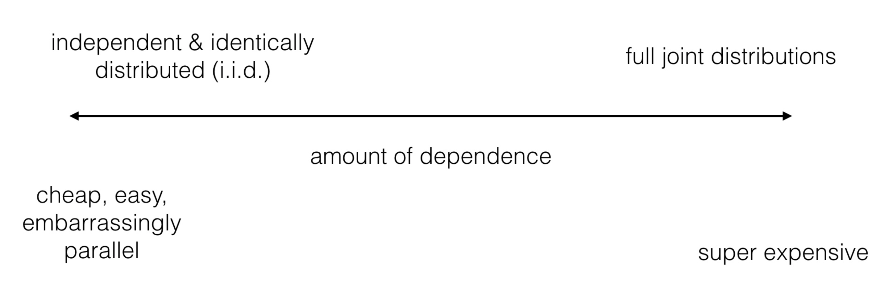
- Graphical models: allow us to be somewhere in the middle.
- Time series data: self-driving sensor readings over time, stocks, weather.
- Relation across time.
- Inference with TS data:
- Predict the future
- Filtering/smoothing: observe noisy data from sensors and find a truer form of data
Definition 1 (Markov assumption) The past is independent of the future given the present. t+1 only depends on t. Mathematically:
\[ p\left(x_1, \ldots, x_T\right)=p\left(x_1\right) \prod_{t=1}^{T-1} p\left(x_{t+1} \mid x_t\right) \]
- Important to understand the idea behind the general form above. It states that if we are at time step \(t=7\), we only need to condition on \(t=6\) rather than \(t={1,2,3,4,5}\). This is the Markov assumption (similar to the conditional independence assumption made in BN’s).
- The previous information is simply encoded within the priors. We multiply the current \(p\left(x_{t+1} \mid x_t\right)\) by all the previous ones (priors).
Example:
\[ p\left(x_1, x_2, x_3, x_4\right)=p\left(x_1\right) p\left(x_2 \mid x_1\right) p\left(x_3 \mid x_2\right) p\left(x_4 \mid x_3\right) \]
We get the whole joint!
Summary: markov models are a type of PGM to represent large joint distributions compactly where there is no directed edges (no conditional dependence). Instead, we compactify the joint via the markov assumption: that the next state only depends on the current state, multiplied by the priors of the previous states. This is useful for temporal and sequential data. We can perform inference via forward message passing and variable elimination.
Inference
To perfrom inference (determining the value of a random vaiable(s)) with Markov models, we use variable elimimation or forward message passing. In general, the goal of inference is to compute the conditional probabilities of certain variables in the model given some observed evidence. This involves using the graphical structure of the model and the associated probabilities to propagate information and make predictions.
- VE/FMP is like dynamic programming. We have the full markov model joint:
\[ p(X)=p\left(x_1\right) \prod_{t=1}^{T-1} p\left(x_{t+1} \mid x_t\right) \]
and we want to perform inference which means computing the probability for some variable \(p\left(x_{t+1}\right)\). To do this traditionally, we’d have to do;
\[ p\left(x_4\right)=\sum_{x_1, x_2, x_3} p\left(x_1\right) p\left(x_2 \mid x_1\right) p\left(x_3 \mid x_2\right) p\left(x_4 \mid x_3\right) \]
where we sum over all the possible states for \(x_1, x_2, x_3\). This is massive computation. FMP states that we can eliminate variables recursively:
we know from above that
\[ p\left(x_2\right)=\alpha_2\left(x_2\right)=\sum_{x_1} p\left(x_1\right) p\left(x_2 \mid x_1\right) \]
and so we store \(p\left(x_2\right)\) in a memoization table. and then we propogate upwards to our desired value:
\[ p\left(x_3\right)=\alpha_3\left(x_3\right)=\sum_{x_2} \alpha_2\left(x_2\right) p\left(x_3 \mid x_2\right) \]
see how we hash \(\alpha_2\) in our computation for \(p\left(x_3\right)\)? This avoids the need for recursive computation. Finally:
\[ p\left(x_4\right)=\sum_{x_3} \alpha_3\left(x_3\right) p\left(x_4 \mid x_3\right). \]
More generally, we have:
\[ p\left(x_{t+1}\right)=\sum_{x_t} p\left(x_t\right) p\left(x_{t+1} \mid x_t\right). \]
Of course, inference extends beyond blind probabilies. We can observe some evidence in the real world and now determine the probability of the marginal \(p\left(x_4 \mid x_1=1\right)\) for example. Even more interesting: observing a future state \(p\left(x_4 \mid x_1=1, x_8=0\right)\).