Final Review Document
I. Constraint Satisfication Problems
- If we take that the factors of the factor graph are constraints that result in 0 if not satisfied, then satisfiable assignments will have a weight > 0 because if at least one constraint is not satisfied, then the whole multiplication goes to 0. So the objective of maximizing the weight holds here.
II. Markov Networks
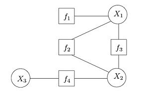
- Factor graphs: basically bipartie undirected graphs where there exists nodes representing RV’s and nodes representing factors which are functions acting on the RV’s they are connected to. Factors are simply functions which spit out some scalar value given assignments to the RV’s they take in. Here is an example:
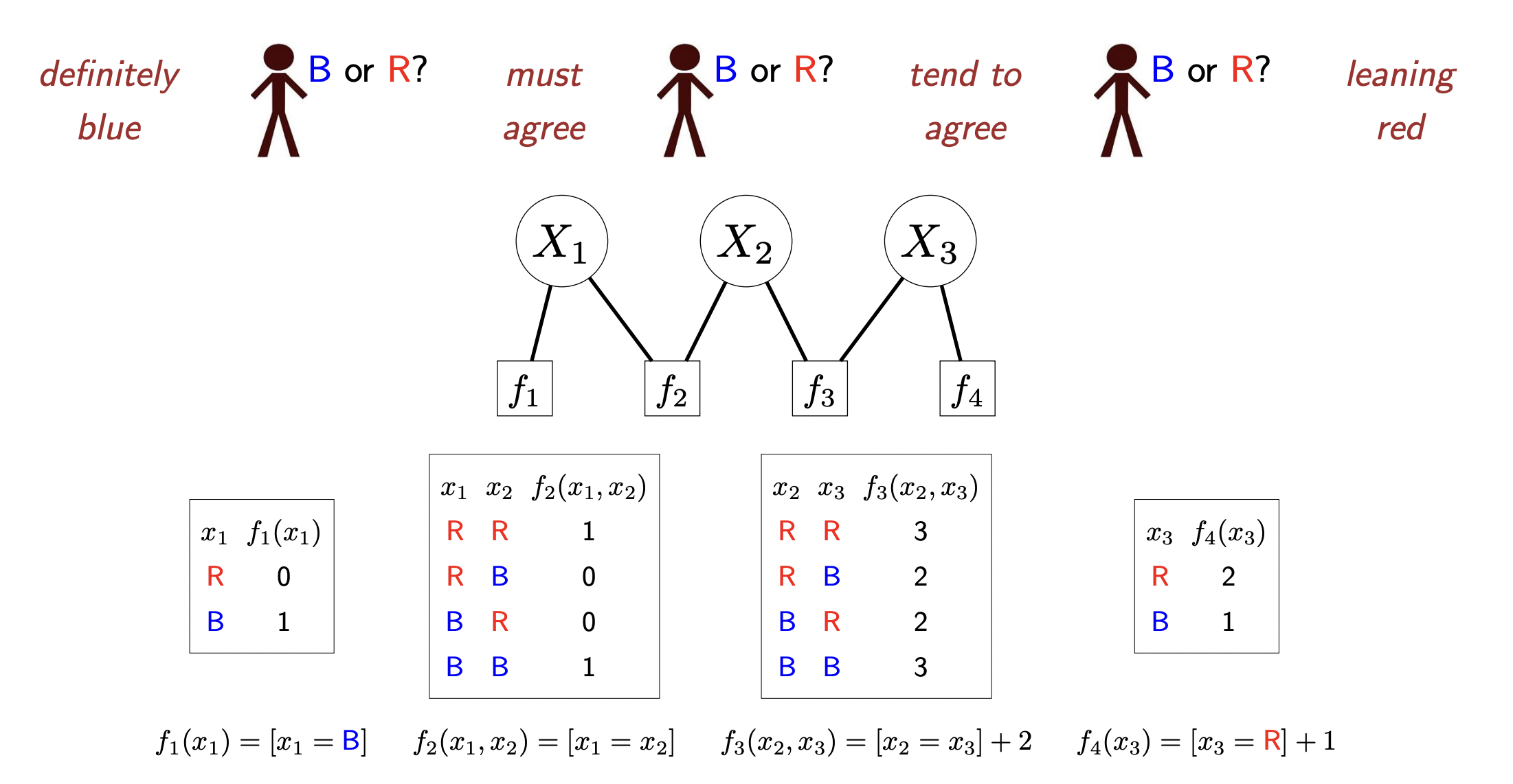
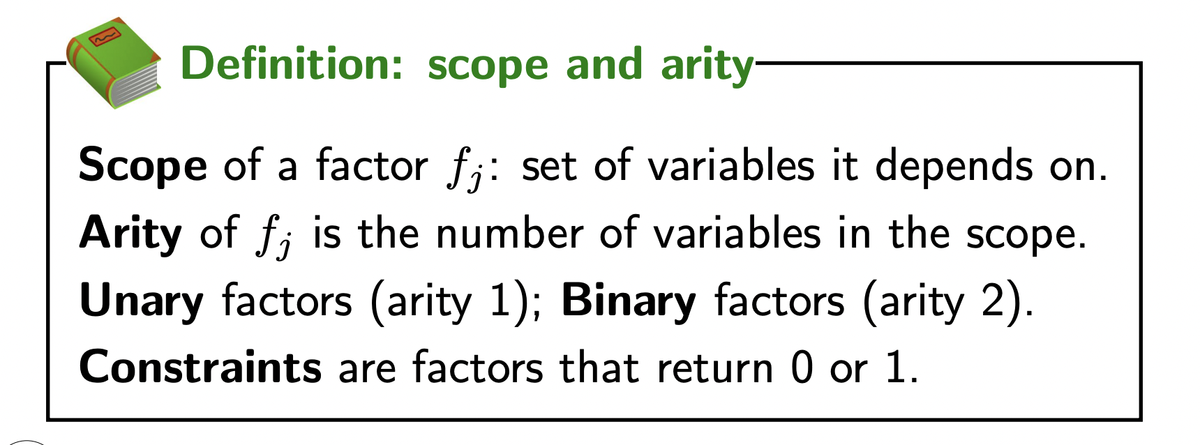
Some useful terms for factors:
each assignment of values to the RV’s has a weight associated to it which involves multiplying the factors together:
Definition 1 (Assignment weights) Each assignment \(x=\left(x_1, \ldots, x_n\right)\) has a weight: \[ \operatorname{Weight}(x)=\prod_{j=1}^m f_j(x) \]
Transitioning to markov networks
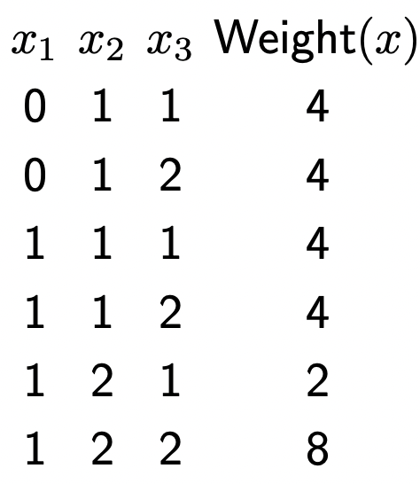
- Markov networks are just factor graph’s but with probability defined to each assignment of the variables rather than weight. Before, we’d have a table that looks like this which specifies a weight for each assignment:
- Now, we can normalize it by dividing each weight by the sum of all weights:
\[\mathbb{P}(X=x)=\frac{\text { Weight }(x)}{Z}\]
where \(Z=\sum_{x^{\prime}}\) Weight \(\left(x^{\prime}\right)\). We now have:
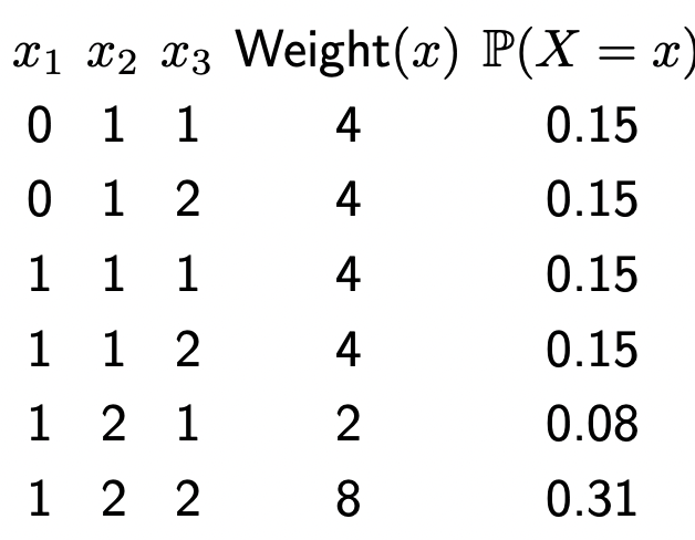
this allows us to represent uncertainty. We can perform inference via taking marginals for example.
\[ \begin{aligned} & \mathbb{P}\left(X_2=1\right)=0.15+0.15+0.15+0.15=0.62 \\ & \mathbb{P}\left(X_2=2\right)=0.08+0.31=0.38 \end{aligned} \]
Note: different than max weight assignment!
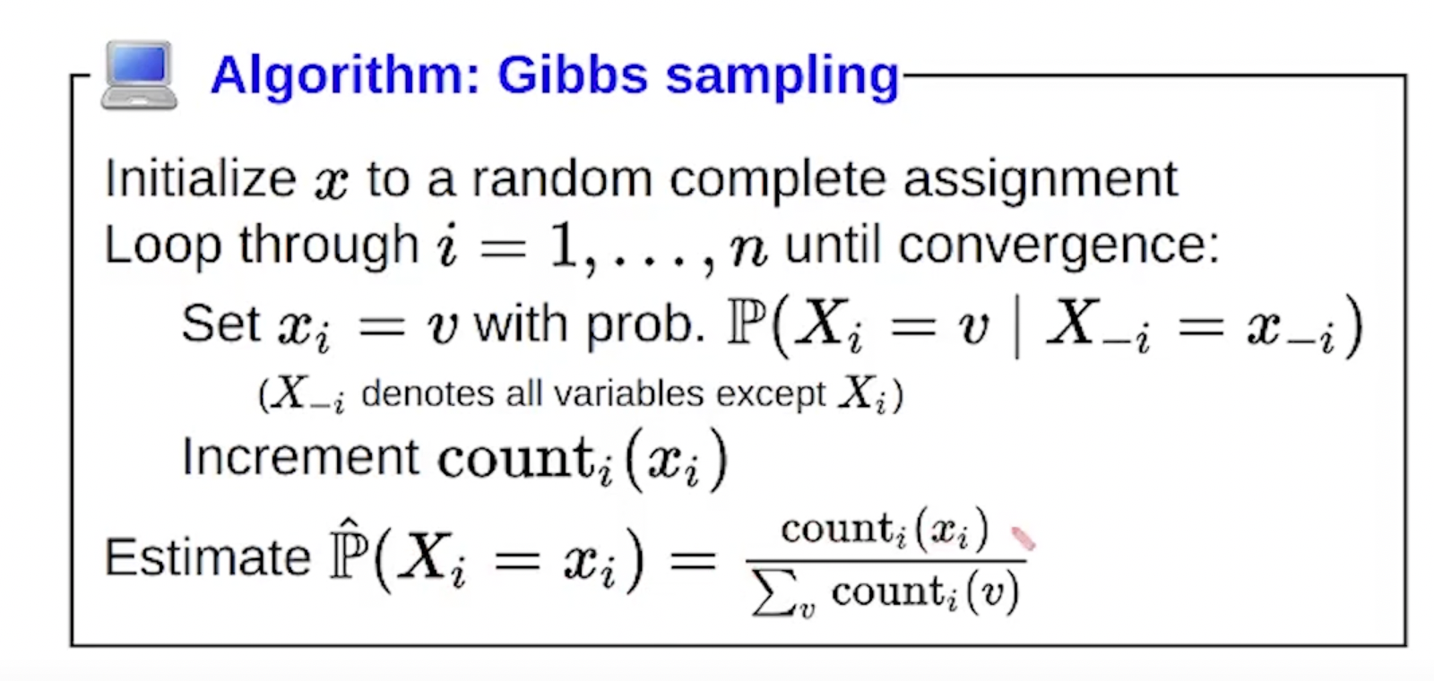
Gibbs Sampling
- We are interested in computing marginal, conditional, and regular probabilities from the distribution that the markov network represents. Here, we discuss an inference algorithm to approximate the marginal calculations (e.g., what is the probability of some random variable \(X_2\)?).
- Marginal probabilities are computed by summing the probabilities over all assignments satisfying the given condition. Gibbs sampling gives us a computationally efficient approximate.
- Note: only given conditional probabilities rather than marginal in the graphs so we must approximate it.
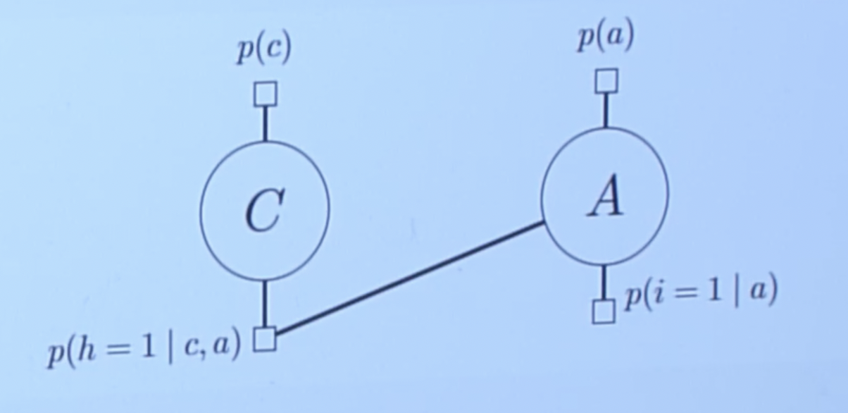
- Cond probs are represented by the factors which are often derived when converting bayesian to markov:
Describe algorithm steps here.
III. Bayesian Networks
- Form of modeling the world. A BN is simply a directed acyclic graph of random variables where directed edges between nodes represents conditional dependence and causation.
- Joints are too big in the real world. Can’t:
- Efficiently store all the combinations. We’d have \(2^k\) parameters where \(k\) is the number of RV’s.
- Perform useful inference due to the global nature of the joint.
- Bayes nets allow us to compactly represent the joint via local conditional probability distributions for each RV. And it resolves the second problem by reasoning locally but conditioning globally. This relies on two concepts:
- conditional independence
- chain rule
The full joint would be to multiply the RV’s out:
\[ P\left(x_1, x_2, \ldots x_n\right)=\prod_{i=1}^n P\left(x_i \mid x_1 \ldots x_{i-1}\right) \]
this is true for any distribution (this is just the chain rule). However, in bayes nets, we assume conditional independence meaning each node is conditionally independent from every node buts its parents. So we reduce the above to:
\[ P\left(x_i \mid x_1, \ldots x_{i-1}\right)=P\left(x_i \mid \operatorname{parents}\left(X_i\right)\right) \]
which still gives us a valid joint:
\[ P\left(x_1, x_2, \ldots x_n\right)=\prod_{i=1}^n P\left(x_i \mid\right. \text{parents}\left.\left(X_i\right)\right) \]
See how much space we save by making the conditional independence assumption?
Conditional Independence
- Main characteristic that allows us to formulate joints via Bayes’ nets. Essentially, conditional independence allows us to condition only on the local parents for each node rather than the ancestor variables.
Example:
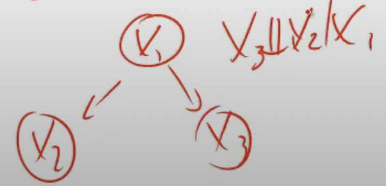
\(x_3\) is independent of \(x_2\) given \(x_1\).
Important points
- You can recover the full joint from a Bayes net via chain rule:
\[ P\left(x_1, x_2, \ldots x_n\right)=\prod_{i=1}^n P\left(x_i \mid\right. \text{parents} \left.\left(X_i\right)\right) \]
- Inference in a Bayesian network involves computing the probability of a variable, or a set of variables, given some evidence. This involves combining the probabilities of the variables using the chain rule of probability and the conditional probabilities represented in the network.
- Factors in a Markov network may include variables beyond the cliques scope.
- Markov assumption is that the rest of the graph not in the clique is conditionally independent given an observation. As such, the variable only depends on the other variables in its clique.
- clique means subgraph where each vertice is adjacent. That is, every markov inference is conditioned on its neighbors only.
- In other words:
- Any two non-adjacent variables are conditionally independent given all other variables… aka Any variable is conditionally independent of the other variables given its neighbors.
- In other words:
- clique means subgraph where each vertice is adjacent. That is, every markov inference is conditioned on its neighbors only.
- The probability is \(p\left(x_1, \ldots, x_n\right)=\frac{1}{Z} \prod_{c \in C} \phi_c\left(x_c\right)\) which means it sums \(\sum_{x_1, \ldots, x_n}\) over all values in the given inference. For example, you have to set of assignments to the variables \(x_1, \ldots, x_n\) and so you calculate the probability that this prediction is correct based on the given formula. But you sum the factors for normalization purposes.
- Here, the probabilities are the factors.
- Can learn the factors (params) via MLE.
- Bayesian to Markov:
- Draw edges between all parents for each given node (go one by one).
- Remove directionality
- Factor graphs:
- bipartite graph. One type of vertex is factor and another RV. Edges connect the factors to the variables such that the edges connect the variables that the factor depends on. Example:
Inference:
- Two types:
- Marginalization: what is the probability of a given variable in our model after we sum everything else out (e.g., probability of spam vs. non-spam)?: \(p(y=1)=\sum_{x_1} \sum_{x_2} \cdots \sum_{x_n} p\left(y=1, x_1, x_2, \ldots, x_n\right)\).
- Maximum a posteriori (MAP) inference: what is the most likely assignment to the variables in the model (possibly conditioned on evidence)?: \(\max _{x_1, \ldots, x_n} p\left(y=1, x_1, \ldots, x_n\right)\).
- Sometimes computationally intractable.
- Two types:
Sampling-based inference:
- Exact inference is often too slow for large distributions. So we need to approximate using sampling methods.
- variational: inference by solving some optimization problem.
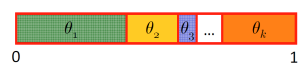
- Sampling: produce answers by repeatedly generating random numbers from a distribution of interest.
- Sample meaning: for example, divide the space into areas with sizes representing the corresponding probabilities. Throw a dart randomly at it:
- Sampling from a Bayes net:
- Sample each variable, conditioned on its parents, which will be observed if you go…, in topological order. Linear time. Topological order means start with node of no parents (i.e., conditioned on nothing), then sample on its children which will be sampled on itself the parent, then work your way down. See forward sampling section here.
- Gibbs sampling: say we want to compute assignments to the variables \(x_1, \ldots, x_n\). We are given a markov network with factors representing transition probabilities. E.g.:
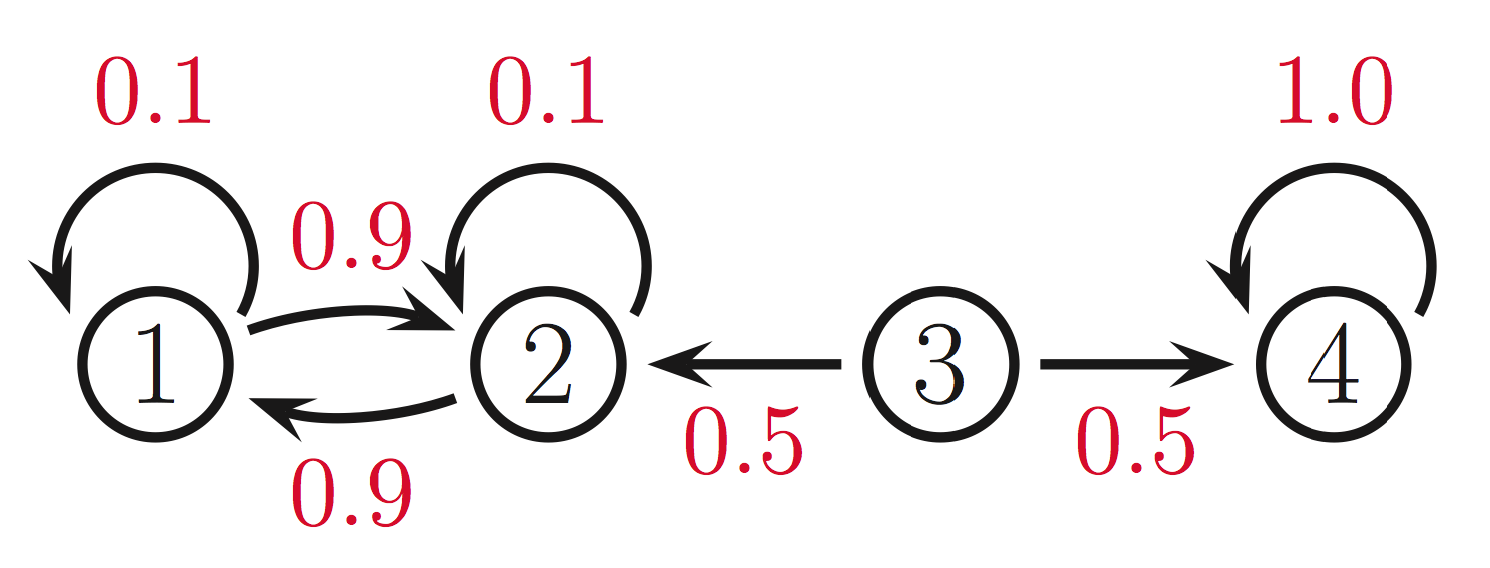
- Set the variables to some random initial state for \(t=0\): \(x^0=\left(x_1^0, \ldots, x_n^0\right)\).
- For \(t\) time steps, we want to update these assignments. Repeat the following \(t\) times:
- Let \(x \leftarrow x^{t-1}\) where \(x\) represents \(x^t\), the assignment of variables that we are currently updating.
- Loop through all variables:
- Sample \(x_i^{\prime} \sim p\left(x_i \mid x_{-i}\right)\) where \(x_{-i}\) means all variables except \(x_i\).
- IMPORTANT: due to the markov assumption, \(x_{-i}\) reduces to \(x_i\)’s neighbors (its clique)! So we only really condition on its neighbors rather than everything else.
- Update the global vector \(x \leftarrow\left(x_1, \ldots, x_i^{\prime}, \ldots, x_n\right)\).
- Sample \(x_i^{\prime} \sim p\left(x_i \mid x_{-i}\right)\) where \(x_{-i}\) means all variables except \(x_i\).
- Set \(x^t \leftarrow x\).
Some notes:
- Sampling is only conditioned on neighbor nodes.
- Note that when we update \(x_i\), we immediately use its new value for sampling other variables \(x_j\).
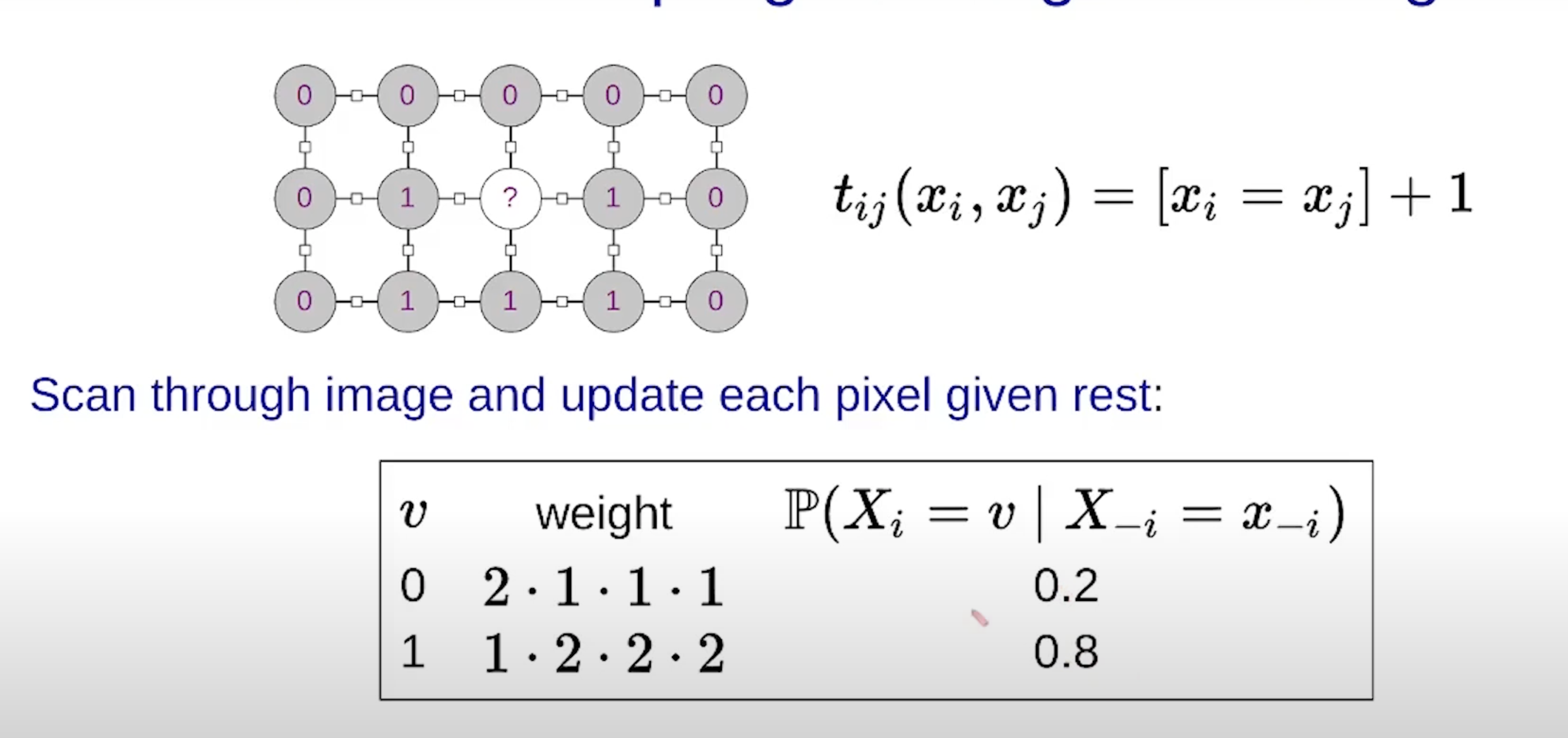
- Often times, you are not given a conditional probability distribution exactly (cuz otherwise no need for sampling just use the joint) for each variable. Instead, you’ll be given factors. So to get probabilities, loop over all possible combinations of \(x_i\) and assign each a weight given the factors (put assignment into factor). Then sample from that probability distribution:

- Only use factors in clique?
This picture sums it up perfectly:
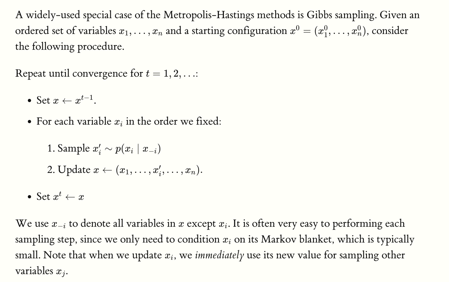
Note… the algo presented in class in slightly different and just counts the number of times the variable \(x_i\) was set to some value and then normalizes:
Note: it seems that for marginal we only compute the weights and probabilities for the clique and factors that touch the RV \(x_i\):
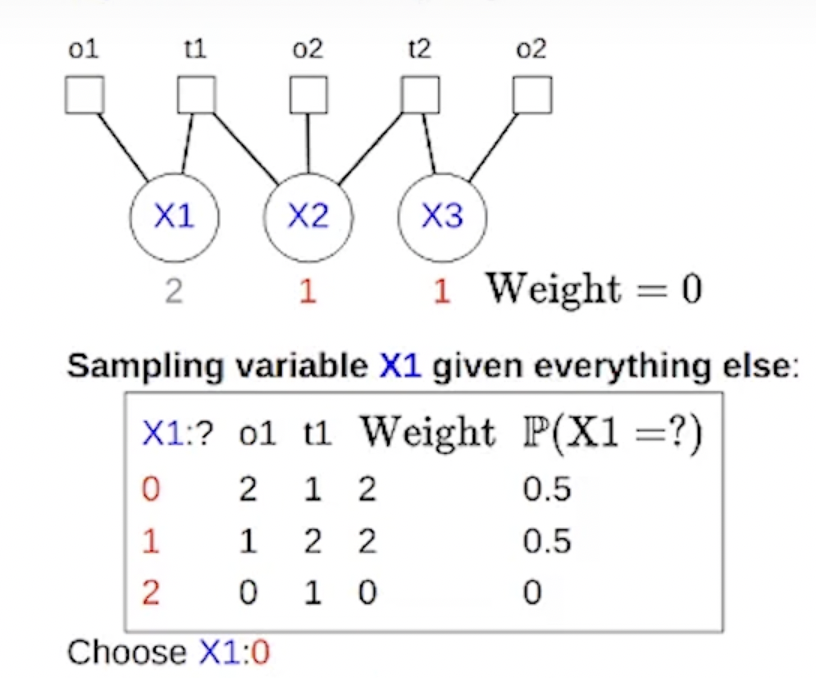
- Another note: you may think that when we loop through all possible values for \(x_i\) to perform the inputs into the factors, we’d have to loop through all the other inputs variables in the factors’ scopes. This is not true because we are operating under the assumption that the neighboring variables have been observed already and thus have a concrete value (e.g., image denoising). Example:
- Parameter learning: where the graph structure is known and we want to estimate the factors (i.e., the probabilities) from data sets.
Questions
- Why do we assume conditional independence in Bayesian networks? That is, why do we assume that the value of each node depends only on its direct parents rather than the rest of the network and/or its ancestors?
- I think this is just the assumption we make when modeling the world using Bayes nets.
- We assume the “markov property”.