CS 228 Notes
This document contains my notes for the CS 228 concepts relevant for CS 221. Mainly following https://ermongroup.github.io/cs228-notes/representation/directed/.
I. Bayesian Networks
- BN’s show casuality, MRF’s cannot.
- Models the world via DAG and efficiently parameterizes a probability distribution.
- We can compactly represent the joint using a Bayes net via the following derivation:
By chain rule, we can represent any joint like so:
\[ p\left(x_1, x_2, \ldots, x_n\right)=p\left(x_1\right) p\left(x_2 \mid x_1\right) \cdots p\left(x_n \mid x_{n-1}, \ldots, x_2, x_1\right). \]
If we make the conditional independence assumption that each factor/variable depends only on a few ancestor variables, then we have:
\[ p\left(x_i \mid x_{i-1}, \ldots, x_1\right)=p\left(x_i \mid x_{A_i}\right). \]
this might allow us to, for example, reduce \(p\left(x_5 \mid x_4, x_3, x_2, x_1\right)\) to \(p\left(x_5 \mid x_4, x_3\right)\) operating on the conditional independence assumption that \((x_5 \mid x_4, x_3) \perp (x_2, x_1)\).
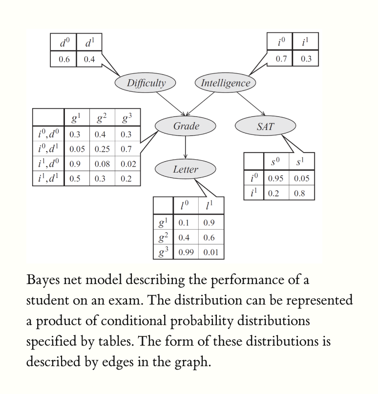
- We can think of \(p\left(x_i \mid x_{A_i}\right)\) as a factor or distribution and denote it using a probability table where rows correspond to the different assignments \(x_{A_i}\) can take on and the columns can correspond to the value of \(x_i\) which denote the actual probabilities for \(p\left(x_i \mid x_{A_i}\right)\) given the rows.
- That is, we can think of each node as a factor/distribution, conditioned on its ancestors.
Bayesian networks reduce the space complexity (size of joint table) from
\[O\left(n d^{k+1}\right)\]
to
\[O\left(d^n\right)\]
where each of the \(n\) variables can have up to \(k\) ancestors and take on one of \(d\) values.
Say we have 5 random variables. The traditional joint table would be huge. But with conditional independence assumptions, we can, for example, have this:
Bayes nets give us a much smaller way to represent this!
A bayesian network is a method to compactify a joint probability distribution relying on the (causal) conditional independence assumption, \(P\left(x_i \mid x_1, \ldots x_{i-1}\right)=P\left(x_i \mid \operatorname{parents}\left(X_i\right)\right)\) that is able to display causal relationships. Formally, a bayesian network is a directed graph \(G= (V, E)\) together with
- A random variable \(x_i\) for each node \(i \in V\).
- One conditional probability distribution (CPD) \(p\left(x_i \mid x_{A_i}\right)\) per node, which specifies the probability of \(x_i\) conditioned on its parents’ values.
- Each node can be thought of as a probability distribution whose value depends on the assignments given to its parent nodes.
- Importantly, the graph must be acyclic otherwise the causality and conditional assumptions are invalid. More importantly then, the distributions may not sum to 1 and therefore be invalid probability distributions.
Conditional independence
Before we move on, we need to drill down the concept of conditional independence. We will introduce it with an example. CI allows us to make assumptions described below which allows us to draw bayes nets which in turn allows us to reduce the joint size.
Example 1 (Conditional independence example with university admission) Let \(M\) denote whether a student gets into MIT, \(S\) whether a student gets into Stanford, and \(G\) be the student’s GPA. Off the bat, we of course understand that \(S\) and \(M\) depend on \(G\). But one can also reason that, not knowing \(G\), if the student gets into \(M\), then they are a promising student and probably have some increased chance of getting into \(S\) as well even though the two admission processes are separate (see how the \(M\) and \(S\) are not quite independent even though there is no direct causation just correlation?). Now, suppose we observe \(G\) which is the sole determinant for admitting students. Learning that \(S\) is true (1) should not change the result of \(M\) because \(G\) provides all the necessary information. That is, given that we know \(G\), \(M\) is not dependent on (independent) of \(S\). We say that \(M\) is conditionally independent of \(S\) given \(G\). We write:
\[ P(M | S, G) = P(M | G) \]
that is, observing \(S\), given that we have observed \(G\), does not change \(P(M)\).
what this example shows is that \(M\) and \(S\) are not initially independent until \(G\) is observed in which case it then becomes independent. The main premise is that things can be independent/dependent in isolation but change when we observe a new variable. In other words, two events can be independent, but NOT conditionally independent upon observation of some new conditioned on variable. See Wikipedia for examples.
The dependencies of a Bayes net
- To summarize, Bayesian networks represent probability distributions that can be formed via products of smaller, local conditional probability distributions (one for each variable). By expressing a probability in this form, we are introducing into our model assumptions that certain variables are independent.
- This raises the question: which independence assumptions are we exactly making?
There are 3 common structures that exist within Bayes nets (larger ones are just these three common structures stacked):
- Common parent (\(X \leftarrow Z \rightarrow Y\))
- Cascade (\(X \rightarrow Z \rightarrow Y\))
- V-structure (\(X \rightarrow Z \leftarrow Y\))
Visually:
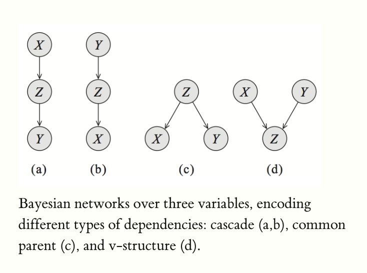
Breaking this down: remember that in a bayes net, each variable is conditionally independent of all nodes in the graph except its parents, given its parents (and the parents are observed). That is, the variable depends directly on its parents. The parents give all the information the variable needs.
- Common parent (\(X \leftarrow Z \rightarrow Y\)):
- If \(Z\) is unobserved, then \(X\) and \(Y\) cannot be deemed independent (they can be dependent)–\(X \not \perp Y\).
- If \(Z\) is observed, then \(X \perp Y \mid Z\) (\(X\) is independent of \(Y\) given \(Z\)).
- \(Z\) contains all the information that determines the outcomes for \(X\) and \(Y\). Once observed, nothing else can affect the outcome. Hence, we have a conditional independence assumption here.
- Cascade (\(X \rightarrow Z \rightarrow Y\))
- \(X \perp Y \mid Z\) (not sure why this is the case)
- Intuition: \(Z\) holds all the information needed for \(Y\). Thus, when \(Z\) is observed, \(Y\) does not depend on \(X\) at all.
- V-structure (\(X \rightarrow Z \leftarrow Y\))
- explaining away
- \(X\) and \(Y\) are independent when \(Z\) is unobserved.
- \(X \not \perp Y \mid Z\) if \(Z\) is observed.
- Opposote of common parent (common child essentially)… but this flips the conditional independence to false.
V-structure is an important concept. Take an example.
Example 2 (Explaining away) Let \(Z\) be a boolean RV indicating if the lawn is wet. Let \(X\) be if it rains. Let \(Y\) be that sprinkler is on. We have the v-structure: \(X\) or \(Y\) can cause \(Z\). Initially, \(X\) and \(Y\) are independent: knowing if the sprinkler \(Y\) is on, doesn’t alone tell us if it is raining \(X\). However, upon the presence of the lawn being wet, \(Z\), we know that it must have been either raining or the sprinkler is on. Thus, if we know the lawn is wet \(Z\), and we determine that the sprinkler \(Y\) is not on, we can deduce the fact that it is raining \(X\). That is, raining \(X\) is conditionally dependent on the sprinkler \(Y\) given the lawn being wet \(Z\): \(P(X \not \perp Y | Z)\).
So in summary, there exists three common substructures within bayes nets which allow us to make the following condidtional (in)dependence assumptions:
- Common parent (\(X \leftarrow Z \rightarrow Y\)): \[X \perp Y \mid Z\]
- Cascade (\(X \rightarrow Z \rightarrow Y\)): \[X \perp Y \mid Z\]
- V-structure (\(X \rightarrow Z \leftarrow Y\)): \[X \not \perp Y \mid Z\]
This is a nice little technique to determine the conditional independence between two variables upon the presence of a third (a criterion for deciding, from a given a causal graph, whether a set X of variables is independent of another set Y, given a third set Z). ChatGPT gave this explanation:
D-separation works by examining the paths between the two nodes and identifying “blocking” nodes that prevent information from flowing between the two nodes. If there are no such blocking nodes, then the two nodes are dependent; if there are blocking nodes, then the two nodes are independent.
For example, suppose we have a graph with three nodes X, Y, and Z, where there is an edge from X to Y and an edge from Y to Z. In this case, if we want to determine the conditional independence of X and Z given Y, we can use d-separation to examine the paths between X and Z and determine whether there are any blocking nodes.
If we find a path from X to Z that passes through Y, then we can say that X and Z are dependent given Y, because information can flow from X to Y to Z along this path. On the other hand, if we find a path from X to Z that does not pass through Y, then we can say that X and Z are independent given Y, because the presence of Y does not affect the flow of information between X and Z.
Overall, d-separation is a useful tool for determining the independence or dependence of variables in probabilistic graphical models.
II. Markov Random Fields
Some ChatGPT wisdom: However, not every distribution can be represented using a DAG. In particular, a distribution can only be represented using a Bayesian network if it satisfies the Markov property, which states that a variable is independent of its non-descendants given its parents in the DAG.
In some cases, the I-map (mapping of independencies from the actual distribution to the bayes net) cannot be perfect. That is, there can be cases where our bayes net cannot encompass all of the independence assumptions that exist in the underlying distribution. Thus, bayes nets cannot model such a distribution perfectly. Fortunately, we can use undirected graphical models, aka Markov Random Fields, to represent probability distributions where independence assumptions cannot be modeled by directed models.