Week 4, Lecture 1 - Markov Decision Processes I

I. Overview

• Search: model a problem from the world as a graph and find the minimum cost path to solve the problem.
• Search was deterministic.

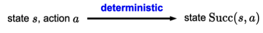
• That is, if we take \(a\) from \(s\), we will always end up in whatever is specified by \(\operatorname{Succ}(s, a)\).
• However, the real world is filled with uncertainty. Take for example, robotic movement. When put in a new environment, there is new uncertainty that we have to tackle.

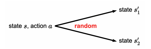
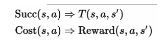
• How to handle such uncertainty? Search in it of itself is not enough. But it provides the basis for MDP’s which allow for uncertainty in \(\operatorname{Succ}(s, a)\).
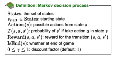
• MDPs: Mathematical Model for decision making under uncertainty.
• Roadmap:

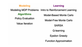
II. Modeling

• Chance nodes: state with action brings us to chance nodes which draws probabilities to the next potential state.
  • Over state and action
• Transition probability: state, action, new state tuple which says, “given a specific state, and an action from that state, what is the probability that we end up in s’?”. Held in a matrix.
• In addition, we also define a reward with the same tuple inputs.
• Goal is to maximize reward (same as minimizing cost just reverse)

More on the transition component:

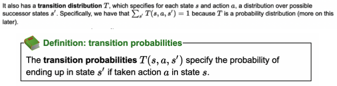
• This makes sense to think of it as a distribution. at each state, given an action from that state, we can end up in different states with different probabilities.
• Instead of having some \(Succ(s,a)\) function that deterministically picks a state given the \((s, a)\) pair, we are instead given a distribution of next possible states with associated probabilities. This distribution of course, must sum to 1.
• What changes from a search problem:

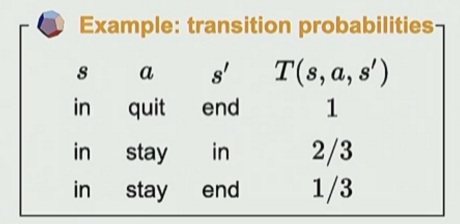
• Example:

In code:

• Change successors and costs function to succProbReward.
  • return list of (newState, prob, reward) triples given (state, action) as input.

class TransportationMDP(object):
    walkCost = 1
    tramCost = 1
    failProb = 0.5

    def __init__(self, N):
        self.N = N

    def startState(self):
        return 1

    def isEnd(self, state):
        return state == self.N

    def actions(self, state):
        results = []
        if state + 1 <= self.N:
            results.append('walk')
        if 2 * state <= self.N:
            results.append('tram')
        return results

    def succProbReward(self, state, action):
        # Return a list of (newState, prob, reward) triples, where:
        # - newState: s' (where I might end up)
        # - prob: T(s, a, s')
        # - reward: Reward(s, a, s')
        results = []
        if action == 'walk':
            results.append((state + 1, 1, -self.walkCost))
        elif action == 'tram':
            results.append((state, self.failProb, -self.tramCost))
            results.append((2 * state, 1 - self.failProb, -self.tramCost))
        return results

    def discount(self):
        return 1.0

    def states(self):
        return list(range(1, self.N + 1))

Policy (the solution)

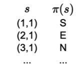
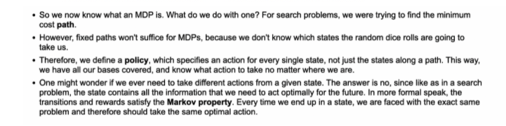
ok cool… what is a solution? In search, we just return the minimum cost path. But here, we must diverge… cuz it isn’t deterministic. Thus, a solution is in the form of a policy.

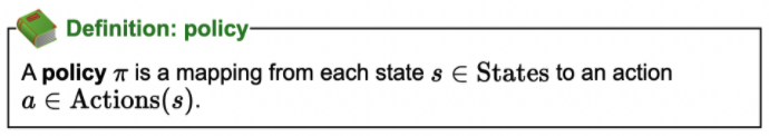
• IT IS A FUNCTION!
  • Takes input, returns output.
  • Takes in each state to an action
  • Lets take this deeper:
    • It may look like this is a path: from each state, we choose the next one. but the key is that they aren’t connected. the states aren’t connected.
    • It just takes in a state, and chooses the best action given that state. It doesn’t draw us to a next state. And this makes sense because we can’t reach the next state deterministically… it happens probabilistically.

💡 Summary: MDP’s add probability to search problems. Imagine nodes in a graph where we start at one state and want to get to some end state. We can take actions at each state but we don’t know which state this will make us end up in. A transition distribution then comes in which specifies, given a state and a corresponding action, returns the corresponding potential new states and the probability that we end up at such a state. To solve an MDP, we can’t specify a path cuz it isn’t deterministic. As such, we specify a policy. A policy is a per-state mapping, which, from each state tells us what action to take (s’ independent).

Ok cool…. we got this gist… now we will talk about how to evaluate policies (are they actually good or not?)

III. Policy Evaluation

• Since we are dealing with non-deterministic scenarios, a policy gives us an inherently ******random****** path. We can never be for certain what path a policy may give us. So to discern whether a policy is good or not, we must built up a framework of knowledge, rooted in probability.
• The goal of an MDP is to maximize the total rewards. To variabalize this, we define this notion of utility:

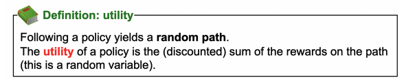
• Inherently, a utility is not deterministic. Thus, we deem it as a random variable and specify a distribution over it (i.e., probability of getting ****this**** reward given the policy).
• So our goal is to maximize the utility. But we can’t maximize a random variable. Thus, we define:

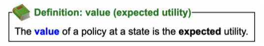
• So really, we wan’t to maximize the ****************expected utility**************** (called the **********value**********).
• So for each policy, we now have a value (expected value for the utility RV) and utility (RV for a policy).
• Example of a utility result:

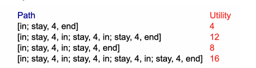
• In sum:

Recall that we’d like to maximize the total rewards (utility), but this is a random variable, so we can’t quite do that. Instead, we will instead maximize the expected utility, which we will refer to as value (of a policy).

• Interestingly, the problem of computing the value of a policy is a complex one. Here, we will discover algorithms for it.

Formal definition:

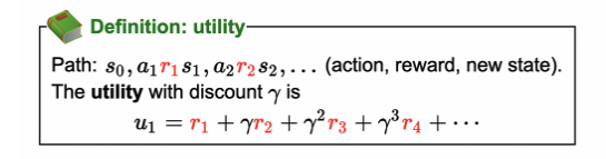
Discount

What the hell is \(\gamma\)?

• To ungreedy-ize this, we introduce discount.
• which captures the fact that a reward today might be worth more than the same reward tomorrow.
  • is discount is small, than favor present more than future. cuz it is between 0 and 1.
• • Note that the discounting parameter is applied exponentially to future rewards, so the distant future is always going to have a fairly small contribution to the utility (unless ).
• • The terminology, though standard, is slightly confusing: a larger value of the discount parameter  actually means that the future is discounted less.

Back to policy evaluation

• We are given a policy, how do we figure out the *****value***** of the policy?

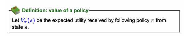
• Function above, given policy and following it from state s, what is the expected utility (value)?
• Let’s bring this up a notch:

• So we see that v_pi(s) gives us value from state s itself.

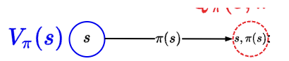
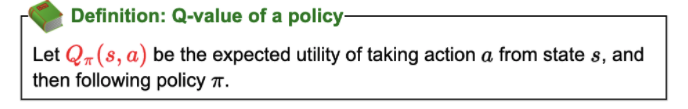
• But what about after state s? state s, given a, will land us in some chance node that points us to different places. but what about chance node to next and so on? Q-value defines this. It is sequential whereas v_pi is one to one.
• It might be hard to understand the difference between \(V_\pi(S)\) and \(Q_\pi(s, a)\). Key differences:
  • \(Q_\pi(s, a)\) takes in both a state and action and plays out the policy. v_pi just takes in state.
    • So as such, q plays out the policy, given that we are taking this next action.
      • See how the math will depend on Q?
• THE BIG RECURRENCE THAT EXPLAINS IT ALL:

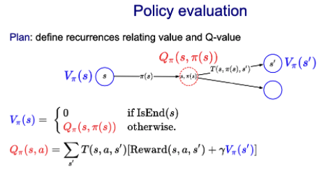
• That is it folks… policy evaluation
• There you have it folks: plug and jug into the equation.
• End node is base case with \(V_\pi( end )=0\).
• See dice game example for solving the closed form of v_pi(in).

Policy evaluation algorithm through iteration

• v_pi is a policy evaluation function: that is, create a mapping (a discrete function) that maps each state to its expected utility (value).

  • Can also do this iteratively with a loop:
    • • Policy iteration starts with a vector (python list) of all zeros for the initial values . Each iteration, we loop over all the states and apply the two recurrences that we had before.

• Run until convergence which we define as:

• \(\max {s \in \text { States }}\left|V\pi^{(t)}(s)-V_\pi^{(t-1)}(s)\right| \leq \epsilon\).

• How to know when to stop? Here is a heuristic:

  • \[\max _{s \in \text { States }}\left|V_\pi^{(t)}(s)-V_\pi^{(t-1)}(s)\right| \leq \epsilon\]

• Note that we only need to keep \(V_\pi^{(t)}\) and \(V_\pi^{(t-1)}\) in the array then because that is all we need to know when we converge.

Summary thus far:

• MDP: graph with states, chance nodes, transition probabilities, rewards
• Policy: mapping from state to action (solution to MDP)
• Value of policy: expected utility over random paths
• Policy evaluation: iterative algorithm to compute value of policy

next… how to find that optimal policy \(\pi\) via value iteration.

IV. Value Iteration

• Given a policy, we know how to know its value \(V_\pi\left(s_{\text {start }}\right)\). But there exists an exponential amount of possible policies (\(A^S\)). So how do we find the optimal one?
• Here, we introduce value iteration, an algorithm for finding the optimal policy. While it may seem that this will be very different from policy evaluation, it is quite similar!

Definition 1 Optimal value: The optimal value \(V_{\text {opt }}(s)\) is the maximum value attained by any policy.

The above definition should be self explanatory: the optimal policy is the one with the highest value.

But it will help us set up the solution. Instead of having a fixed policy for the recurrence like in PE, we will now define a recurrence on top of \(V_{\text {opt }}\) and \(Q_{\text {opt }}\).

Note

Value iteration recurrence:

Optimal value from state \(s\):

\[V_{\text {opt }}(s)= \begin{cases}0 & \text { if IsEnd }(s) \\ \max _{a \in \operatorname{Actions}(s)} Q_{\mathrm{opt}}(s, a) & \text { otherwise. }\end{cases},\]

where the optimal value if take action \(a\) in state \(s\):

\[Q_{\mathrm{opt}}(s, a)=\sum_{s^{\prime}} T\left(s, a, s^{\prime}\right)\left[\operatorname{Reward}\left(s, a, s^{\prime}\right)+\gamma V_{\mathrm{opt}}\left(s^{\prime}\right)\right]\].

Visually:

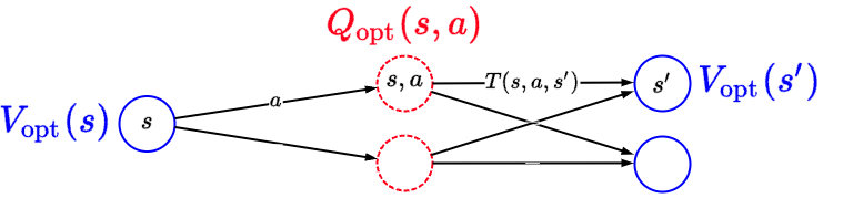
and so then to find the optimal policy, we’d just take \(Q_{opt}\) and do

\[\pi_{\mathrm{opt}}(s)=\arg \max _{a \in \operatorname{Actions}(s)} Q_{\mathrm{opt}}(s, a).\]

Note

Definition 2 (Value iteration algorithm)

1. Initialize \(V_{\text {opt }}^{(0)}(s) \leftarrow 0\) for all states \(s\).
2. For iteration \(t=1, \ldots, t_{\mathrm{VI}}\) :
   1. For each state \(s\) :

\[ V_{\text {opt }}^{(t)}(s) \leftarrow \max _{a \in \text { Actions }(s)} \underbrace{\sum_{s^{\prime}} T\left(s, a, s^{\prime}\right)\left[\operatorname{Reward}\left(s, a, s^{\prime}\right)+\gamma V_{\text {opt }}^{(t-1)}\left(s^{\prime}\right)\right]}_{Q_{\text {oot }}^{(t-1)}(s, a)} \]

• The keen eye will note that this just returns the optimal value and not actually the optimal policy. However, optimal policy comes as a byproduct. Just take the argmax at each state.