Week 3, Lecture 1 - Search I
Date: 10/10/22
I. Overview
We now move into the next unit of the course: Search. This is a reflex-based paradigm. We will still abide by the principles of the “model, learning, and inference” paradigm. To introduce search, take the following canonical problem:
Example 1 (Route planning) Given as the input a map, a source point and a destination point, output a sequence of actions (e.g., go straight, turn left, or turn right) that will take us from the source to the destination. Evaluate based on custom objective (e.g., most scenic route, shortest path, etc.)
- There are many more examples that we can think of. Robot motion planning,solving puzzles, etc. Many traditional (non-ML) algorithmic paradigms (e.g., dynamic programming) make its way into AI through this medium. The main idea though, is that:
- Search problems are defined by their objective and the actions it can take to get there.
Beyond reflex
- Reflex models are very high-level: e.g., classifiers which output a quick “yes” or “no”. Not dependent on any future/past predictions.
- However, some applications of AI (such as solving puzzles), demand more.
- Search problems are an instance of state-based models.
- We are still building a predictor \(f\) which takes an input \(x\), but will now return an entire action sequence, not just a single action (i.e., a “reflex”).
- You can think of the difference as defined by the task. Solving a puzzle is not the same as classifying cats vs. monkeys.
- Can’t you solve a search problem just by iteratively multiplying the reflex-based predictions to get an action sequence?
- Not really… future actions should be conditioned on past actions!
- But… think of this: “if you’re walking around Stanford for the first time, you might have to really plan things out, but eventually it kind of becomes reflex.”.
- We have looked at many real-world examples of this new “search” paradigm. For each example, the key is to decompose the output solution into a sequence of primitive actions. In addition, we need to think about how to evaluate different possible outputs.
Roadmap
- In the ML unit, we had the “model, learning, and inference” paradigm. We adapt this for search too.
- Machine learning:
- Modeling: feature extractor + neural architecture
- Inference: model forward pass (\(f(x)\))
- Learning: algorithms such as stochastic gradient descent to find optimal model weights
- Search: find out down below! We will start with modeling and inference, then learning next lecture.
- Machine learning:
Here is a roadmap of what we will cover:
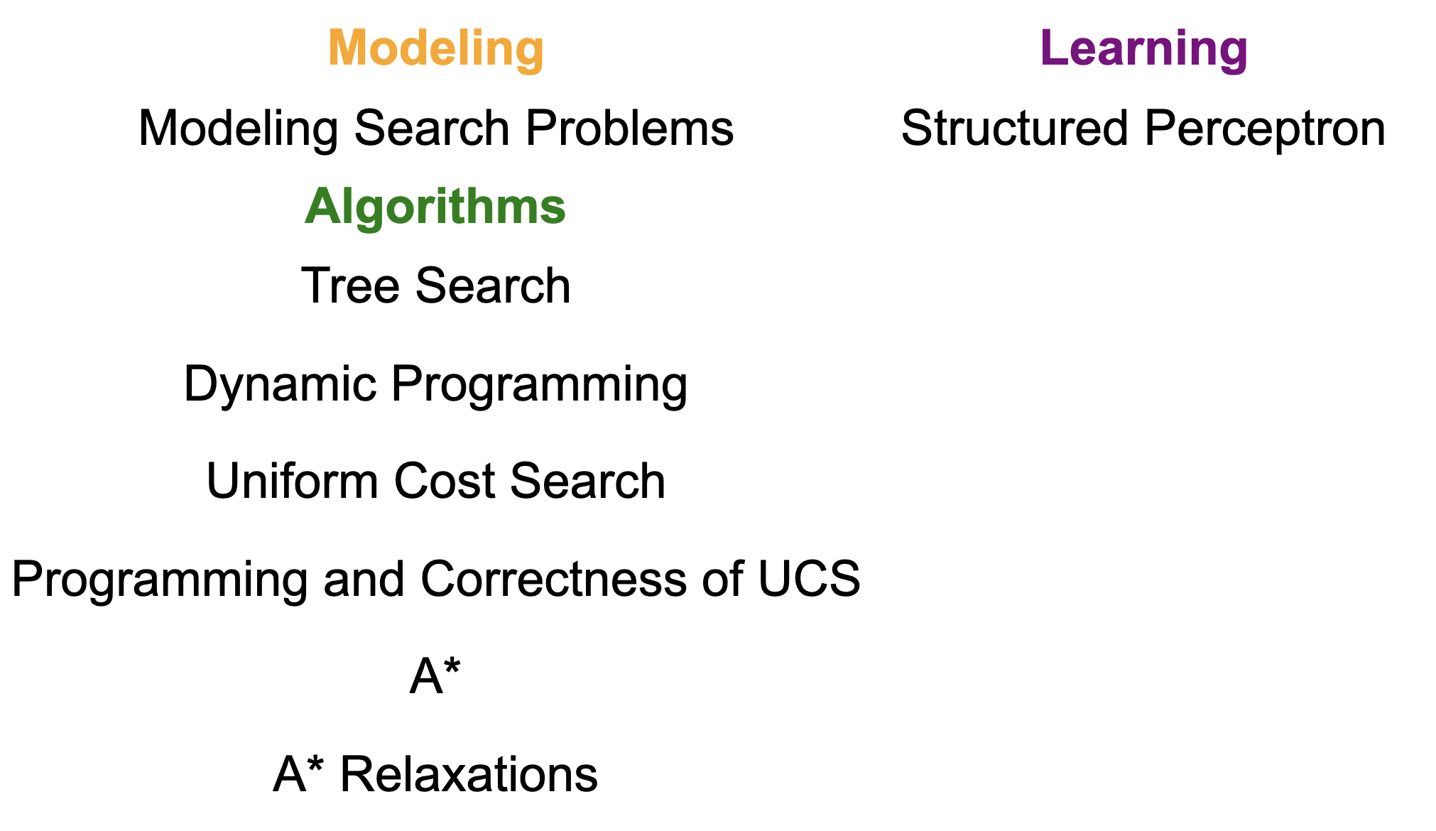
The main idea is to cover how we define (“model”) search problems, and come up with algorithms to solve them.
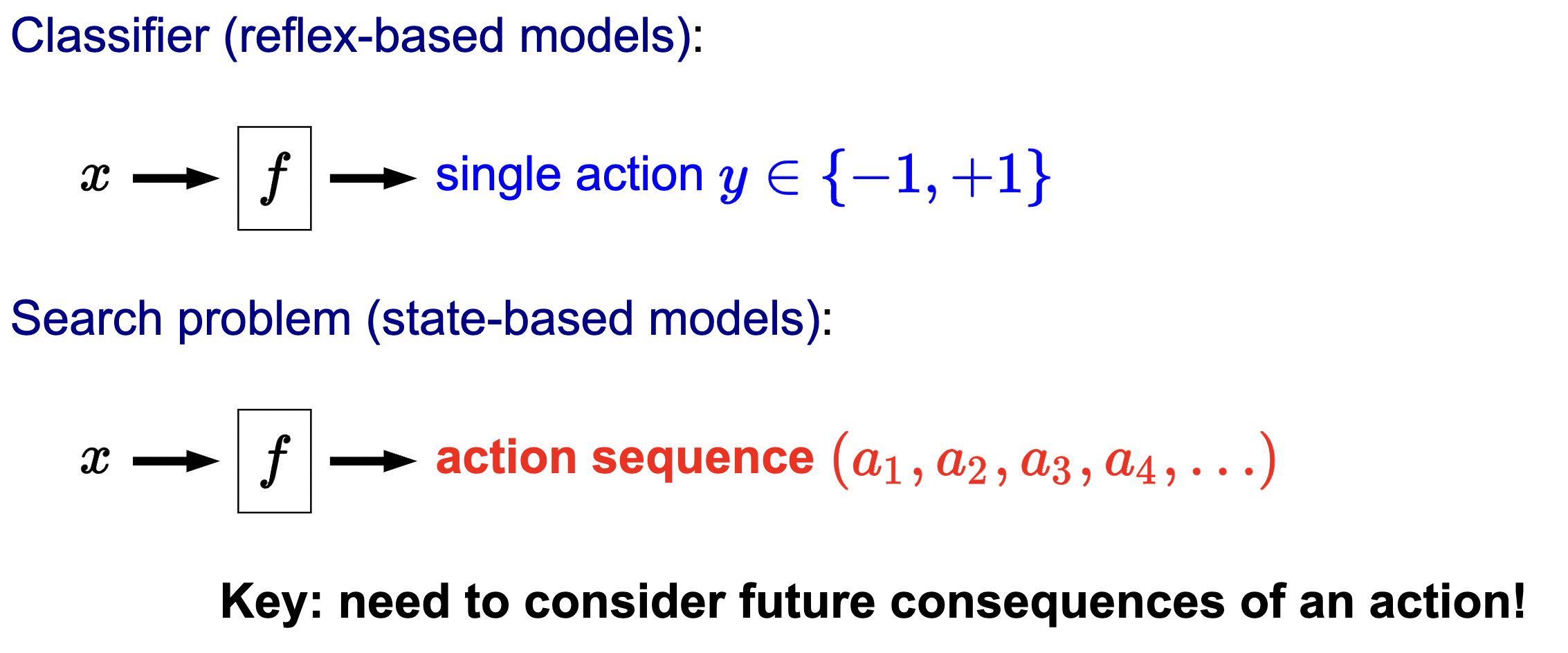
(State-based vs reflex-models) The main TL;DR is to understand the following difference and what problems we can now solve with this new tool:
Reflex-based modeling:
\[ x \rightarrow f \rightarrow \text { single action } y \in\{-1,+1\} \]
(Search) State-based modeling:
\[ x \rightarrow f \rightarrow \text { action sequence }\left(a_1, a_2, a_3, a_4, \ldots\right) \]
This allows us to not only solve things like classification problems with reflex-based modeling, but also now solve things like route planning with state-based modeling.
II. Modeling
Ok… cool! We now have a general intuition for what is search/state-based modeling. Let’s get formal now with definitions.
We will introduce modeling via the following example.
Example 2 (Farmer search problems) A farmer wants to get his cabbage, goat, and wolf across a river. He has a boat that only holds two. He cannot leave the cabbage and goat alone or the goat and wolf alone. How many river crossings does he need?
- You probably thought of each scenario playing out in your head. How can we build a system to do this automatically.
- Search problems define the possibilities, and search algorithms explore these possibilities.
- For this problem, we have eight possible actions, which will be denoted by a concise set of symbols.
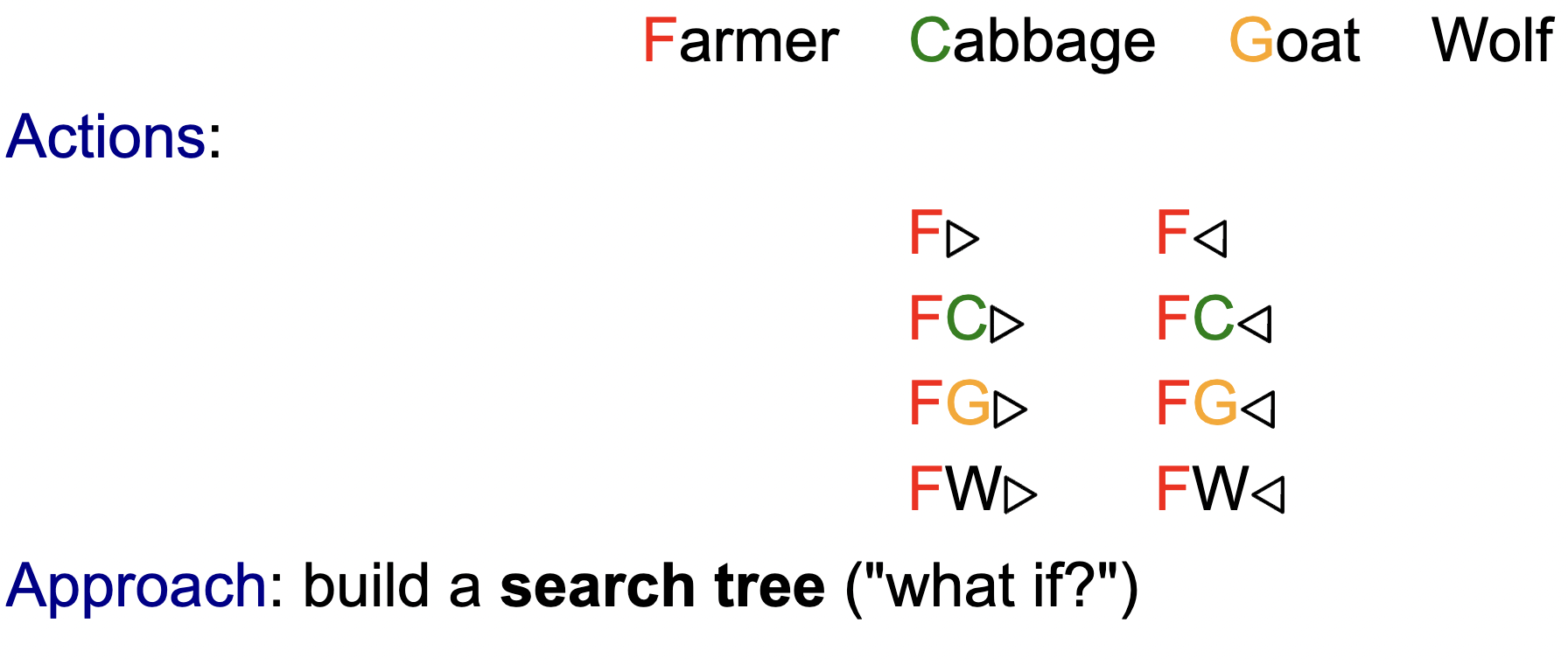
- We can start to build a search tree of each “what-if” scenario. Playing out each scenario, we get the following:
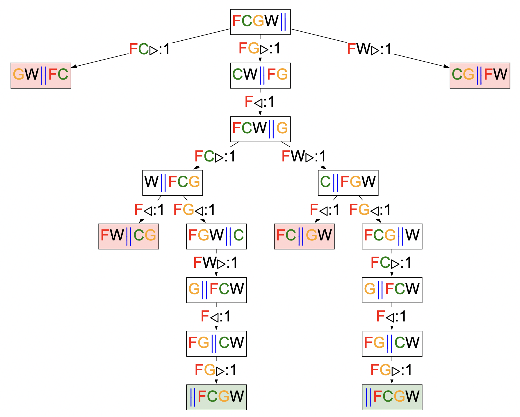
- Each scenario is represented by a “branch” of the search tree.
- We terminate the branch (leaf) once we reached a final state (win or lose).
Let’s formalize this.
Defining the search problem
Definition 1 (Search Problem) A search problem is built upon the following:
- \(s_{\text {start }}\) : starting state
- Actions \((s)\) : possible actions
- \(\operatorname{Cost}(s, a)\) : action cost
- \(\operatorname{Succ}(s, a)\) : successor
- IsEnd \((s)\) : reached end state?
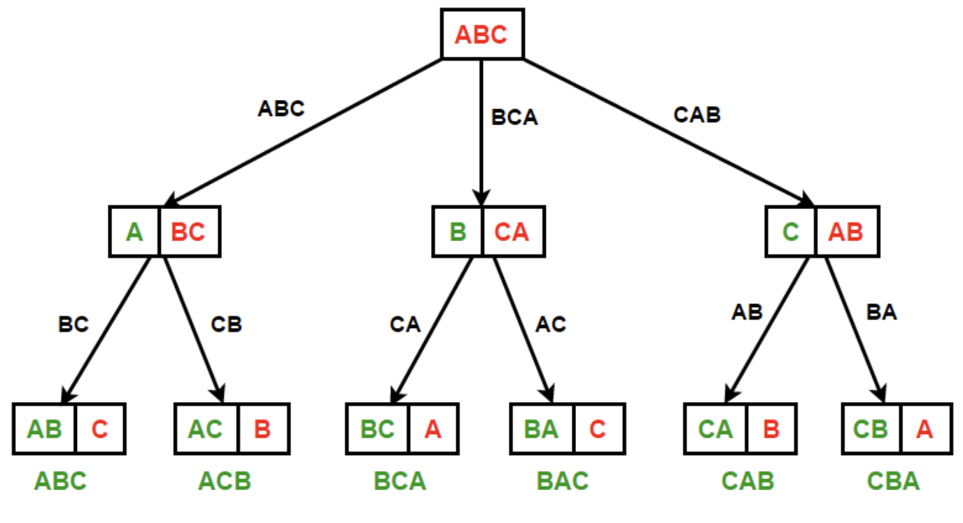
This can be visually represented/solved with a search tree. The root of the tree is the start state \(s_{\text {start }}\), and the leaves are the end states (IsEnd \((s)\) is true). Each edge leaving a node \(s\) corresponds to a possible action \(a \in \operatorname{Actions}(s)\) that could be performed in state \(s\). The edge is labeled with the action and its cost, written \(a: \operatorname{Cost}(s, a)\). The action leads deterministically to the successor state \(\operatorname{Succ}(s, a)\), represented by the child node.
In the example, each root-to-leaf path represents a possible action sequence, and the sum of the costs of the edges is the cost of that path. The goal is to find the root-to-leaf path that ends in a valid end state with minimum cost.
III. Tree search
Cool… we got the formalism and modeling down. Now let’s build algorithms to solve them! We will discuss several tree-based algorithms here.
The idea:
- We have some tree (model) representing the search problem. We want to find paths that lead to successful leaves with the minimum-cost. There are several algorithms that can do this. We can keep track of them via the following factors:
- Algorithm name
- Cost
- Time
- Space
Backtracking
- 106B!
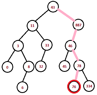
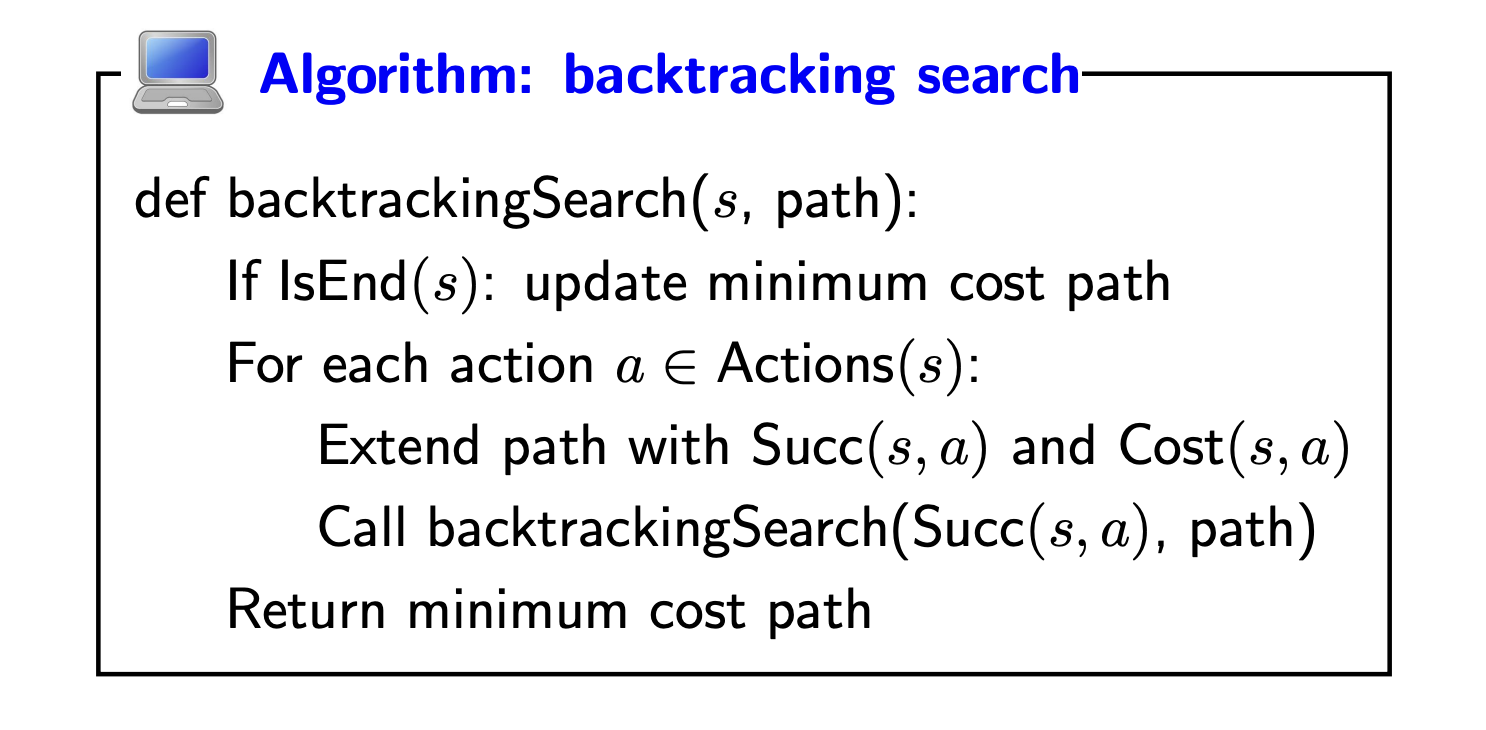
- Brute forces all paths. Basically, just complete depth-first traversal of the search tree and update minimum-cost path along the way.
- We consider all possible actions \(a\) (edges) from state \(s\) (node), and recursively search each of the possibilities, updating the minimum-cost and path along the way.
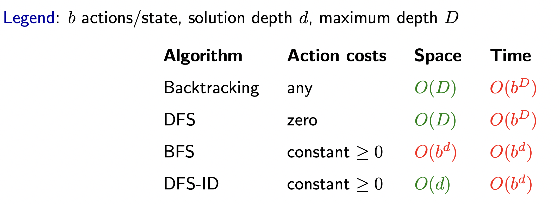
- To get an idea of complexity, we define the following:
- branching factor \(b\): number of available actions at each state1.
- maximum depth \(D\): each path consists of \(D\) or less actions/edges.
- Complexity:
- Space: \(O(D)\)
- Time: \(O\left(b^D\right)\)
- Why \(O(D)\) for space?
- Each path is defined by the sequence of actions you take at each node in the branch. This can be, at the worst, \(D\) long. Example:
- Each path is defined by the sequence of actions you take at each node in the branch. This can be, at the worst, \(D\) long. Example:
- Time also makes sense. We need to search, at worst, \(D\) things for each total branch. But the branching factor \(b\) (a scaling factor), exponentially grows this.
Algorithm:
Depth-first search
Before we go on, let’s do a quick recap:
- State-based modeling allows us to model and solve problems where the output is a sequence of actions to take between states.
- We formalized a search problem via notations such as states and actions.
- We can model a search problem via a tree.
- We can solve a search problem via a traversal algorithm.
- There exists several such algorithms, each differing in performance slightly (some suited for tasks better than others).
Onto DFS:
- Ok… suppose we don’t care about finding the minimum-cost path, but rather simply the first solution path. That is, make the cost \(c = 0\).
- Then, DFS works the best here. Just traverse each branch in a depth-fashion. Stop when you reach the first leaf.
- Time and space complexity is still the same, because, in the worst case, we traverse the whole tree and don’t end up with a solution.
Breadth-first search
- Now suppose all costs of each action are constant. Every action costs \(c\).
- Then, do BFS.
- We traverse the tree laterally.
- When we reach a solution, we know we are at the best one.
- Think about it. If we traverse from the left to the right and find a successful leaf node (successful end state), there can be no branch that is shorter in depth.
IV. Dynamic Programming
- Time-complexity was pretty bad for the tree traversal algorithms for solving search problems. Lots of it is simply too brute-force to be reasonable (at worst case).
- Time-complexity was growing exponentially because we’d have to recurse through the whole maze.
- Let’s see how DP can speed this up.
Here is the general idea:
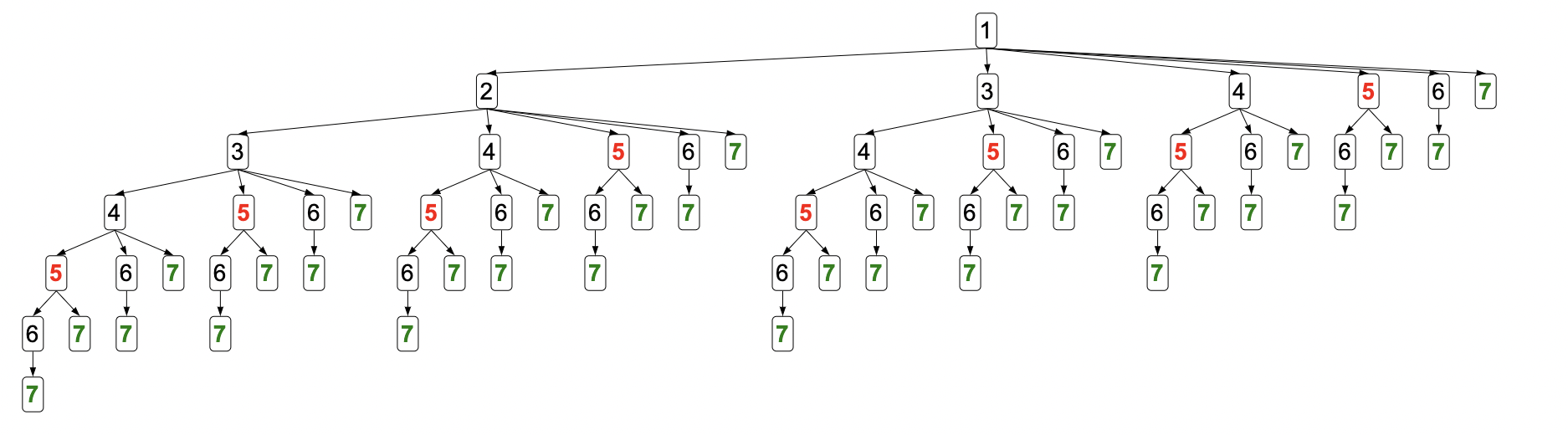
in tree search (take backtracking), we’d have to recurse through each branch, for every branch. Exponential time complexity! However, notice that, for example, once we hit a \(5\), the rest of the branch is the same. This is the key idea. We can store the subproblem path of starting from \(5\) to the solution (leaf) in a lookup table and next time we are at a \(5\), we just look it up! We save tons of time but sacrifice a bit of space while were at it (which is ok!). This concept is called memoization.
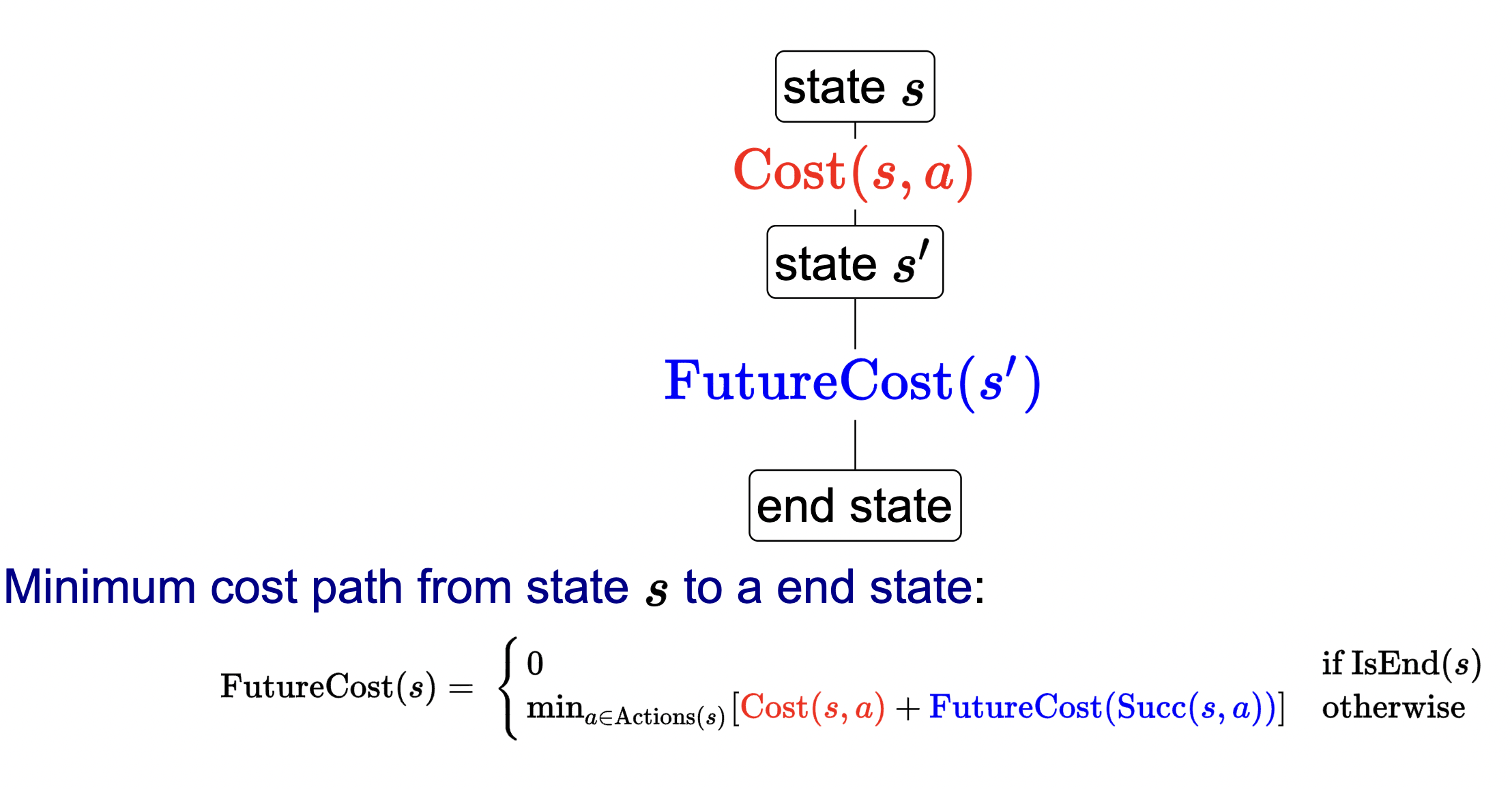
This slide formalizes the concept of dynamic programming.
In code, this would be something like:
if table[subproblem_solution] is not None:
    return table[subproblem_solution]
else:
    # recurse as usual

    # base case
    solution = -1
    if isEnd(state):
        solution = ...
    # recursive step
    for action in actions:
        ...
        solution = ...


    table[subproblem_solution] = solution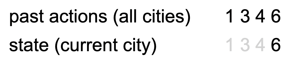
return solution - Key observation is that the future costs only depend on current city… not on what we did in the past to get to that city.
- What we really mean is that future cost only depends on state.
- State goes from “past sequence of actions (e.g.: 1 –> 2 –> 5 –> 6) to just the current thing (e.g.: 6).
- Exponential to polynomial time (based on number of states in polynomial time (\(O(n)\))).
Idea of “state”:
Adding a constraint
Cool… but what happens if we add a constraint dependent on the state.
Example 4 (Route finding) Find the minimum cost path from city 1 to city \(n\), only moving forward. It costs \(c_{i j}\) to go from \(i\) to \(j\).
Constraint: Can’t visit three odd cities in a row.
- Note that we choose what the “state” is in these DP problems. However, time and space complexity is dependent on the size of the state. So choose wisely. A bit of a balance.
- This is why the definition of what “state” is from above makes sense: get the minimal amount of information that you need to know that is sufficient enough to choose actions optimally.
With this constraint in mind, we can now define a new state definition for this problem.
\[ \text{state = (previous city, current city)} \]
example in this context then:
\[S_0:(n / a, 1)\] \[S_1:(1,3)\] \[S_2:(3,7)\]
State space (complexity) is then \(|S|=N \times N=N^2\). We can do better. Define state as:
\[ \text{state = (if previous city was odd, current city)} \]
this gives us \(|S| = 2n\).
The whole example here is to drill in the idea of a “state” and how dynamic it can really be defined (but also how important it is to define a good state).
Acyclic assumption
Definition 4 (Acyclic assumption) The state graph defined by \(\operatorname{Actions}(s)\) and \(\operatorname{Succ}(s, a)\) is acyclic.
Here is a quick primer on the relevant graph algorithm background.
- Acyclic vs. cyclic:
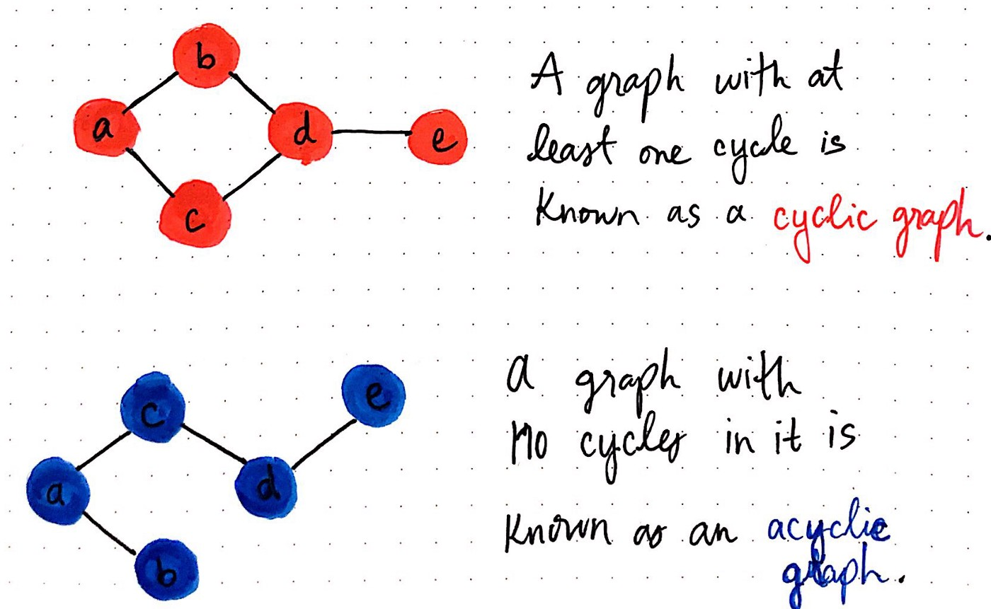
- That is, we need an ordering of the states such that we can’t go “back to a state” to acheive the optimal path.
- So basically, our state graph just has to be acyclic.
- Uniform cost search resolves this.
TL;DR
- DP: backtracking + memoization
- Memoization: cache all solutions to each subproblem. Next time you encounter subproblem, lookup solution in cache instead of redoing the recursion.
- DP offers speed-up in time complexity: exponential to polynomial.
- State: how you define your state plays a huge role in performance. Get the minimal amount of information that you need to know that is sufficient enough to choose actions optimally in the future.
- However, DP depends on the assumption that the graph being traversed is acyclic. That is, there exists some sequential ordering in the problem (no going backwards!).
- Uniform cost search addresses this issue.
V. Uniform cost search
- DP is great, but what happens if we have cycles in our state graph?
- UCS is essentially DP but allows for cycles.
- Basically Dijkstra’s algorithm.
- Again, we will use the following shortest-path example.
Example 5 (Route finding) Find the minimum cost path from city 1 to city \(n\), only moving forward. It costs \(c_{i j}\) to go from \(i\) to \(j\).
- Motivation:
- In DP, we had no cycles, so every future cost only depended on what happens in the future… there is some ordering of the nodes which prevents us from looping backwards to potentially find a more optimal path. The insight is that, once we are at some state \(s\), we know that we got there via the most optimal route from the start state \(s_{start}\). Thus, we only need to consider future costs. Take this visual:
We know that at state \(s\), \(\operatorname{PastCost}(s)\) is optimal; so we can just focus on computing the minimum futuyre cost, \(\operatorname{Cost}(s, a)\). With cycles, this isn’t always the case.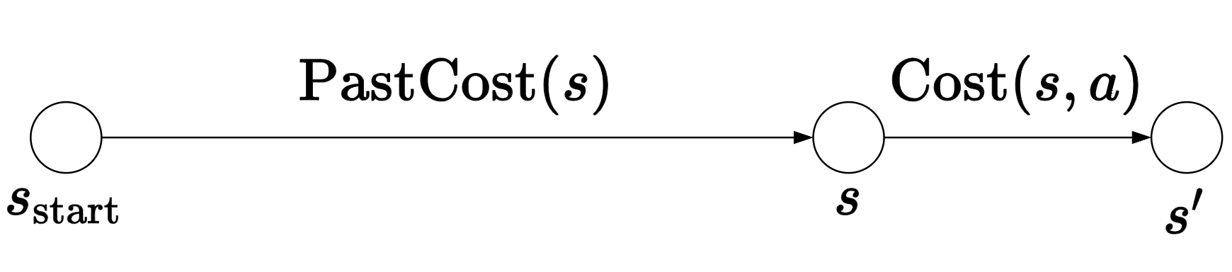
- However, some graphs may have cycles. This introduces the “going backwards possibility to find a potentially more optimal path… and thus complicating the problem.
- Mathematically, also, the difference is that with DP, we computed future costs, but here we can define the compliment: compute \(\operatorname{PastCost}(s)\): the cost of the minimum cost path from the start state to \(s\). Then, we do DP in reverse going from \(s\) to the start state to get the minimum. But again, to use DP, we must ensure that the nodes are computed in order (just reverse this time). But the general idea for USC is to use this “reverse” technique.
- How to solve this? Let’s see what UCS has to offer!
- In DP, we had no cycles, so every future cost only depended on what happens in the future… there is some ordering of the nodes which prevents us from looping backwards to potentially find a more optimal path. The insight is that, once we are at some state \(s\), we know that we got there via the most optimal route from the start state \(s_{start}\). Thus, we only need to consider future costs. Take this visual:
High-level idea:
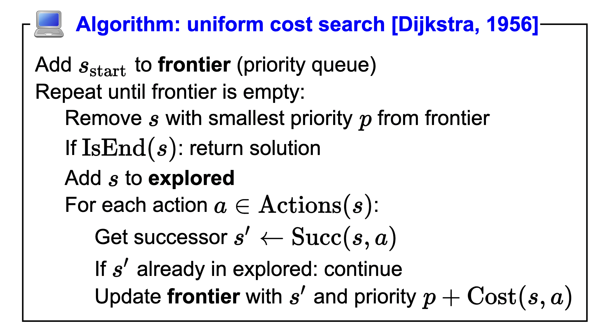
(Key idea of UCS:) UCS enumerates states in order of increasing past cost.
Note that we also assume that all actions (edges) are non-negative (\(\operatorname{Cost}(s, a) \geq 0\)). Bellman-ford resolves this though.
- Quick aside: UCS and Dijkstra’s are practically equivalent algorithmically, but some differences include:
- UCS takes as input a search problem, which implicitly defines a large and even infinite graph. Dijkstra’s takes as input a fully discrete and concrete graph.
- Output difference: Dijkstra’s outputs shortest path between start state and every other node. UCS only does from one desired state to another. 3
Ok… to describe the algorithm, I recommend just watching the video. However, here is some text from the slides.
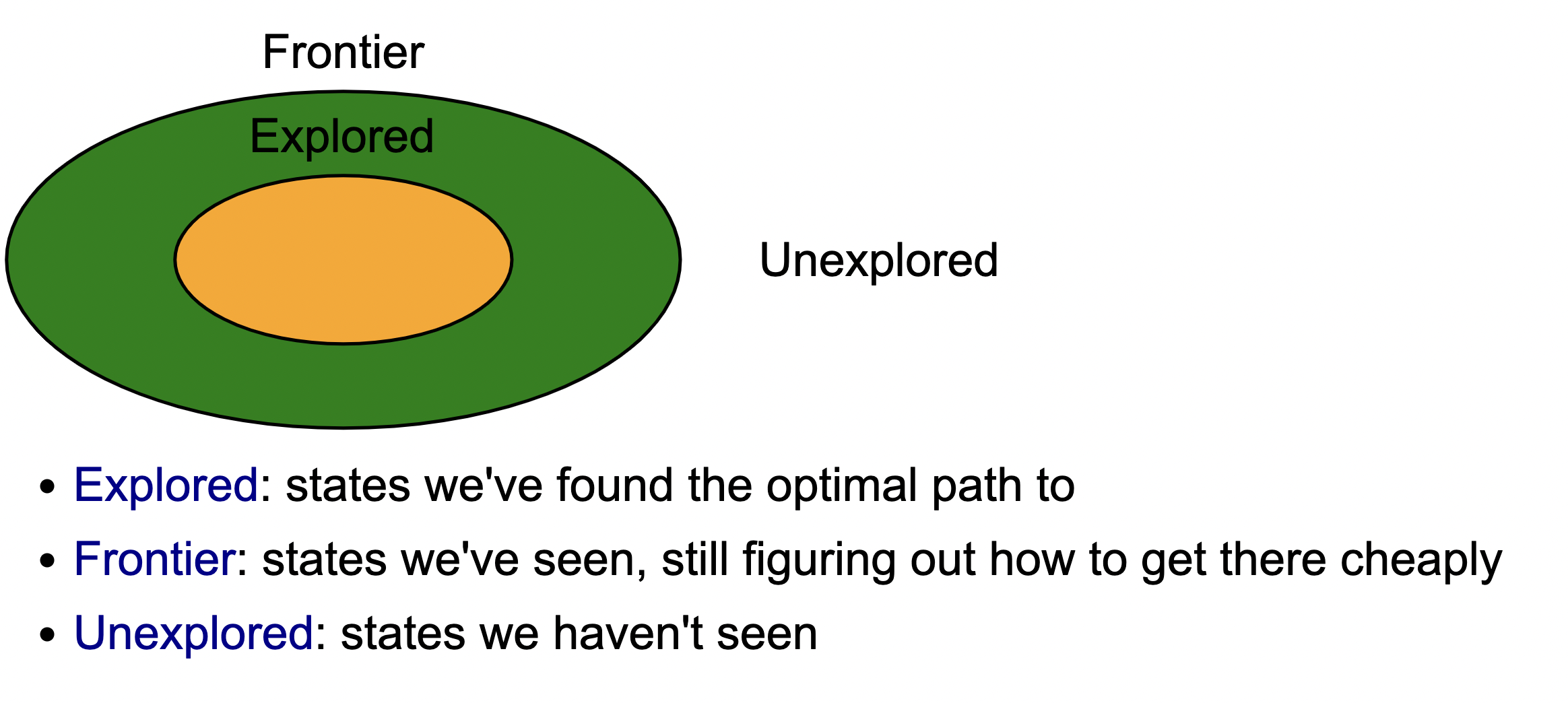
- The general strategy of UCS is to maintain three sets of nodes: explored, frontier, and unexplored. Throughout the course of the algorithm, we will move states from unexplored to frontier, and from frontier to explored.
- The key invariant is that we have computed the minimum cost paths to all the nodes in the explored set. So when the end state moves into the explored set, then we are done.
Also, as another aside before we move on, realize that these algorithms take in state graphs (not trees). Here is a good video walking through an example of this algorithm in a different light.
Notes:
- Once the end state is in explored, we terminate the search.
- Question: can we ever update the minimum cost path to some node already in explored? Or is it true that once a state is in explored, it is already at the minimum cost?
- Ok… the answer is yes (“The key invariant is that we have computed the minimum cost paths to all the nodes in the explored set. So when the end state moves into the explored set, then we are done.”), but I fail to understand why. (update: see below as this is exactly what’s covered next.)
So basically, in Dijkstra’s we do the full graph (end when all nodes are in the graph). In UCS, terminate when the end state is moved to explored.
Ok… I had the following question:
- Is it possible to add a node beyond the desired end state to the frontier and pop that one off to the explored list first? The answer is yes. It is a great exercise to run UCS on the following graph.
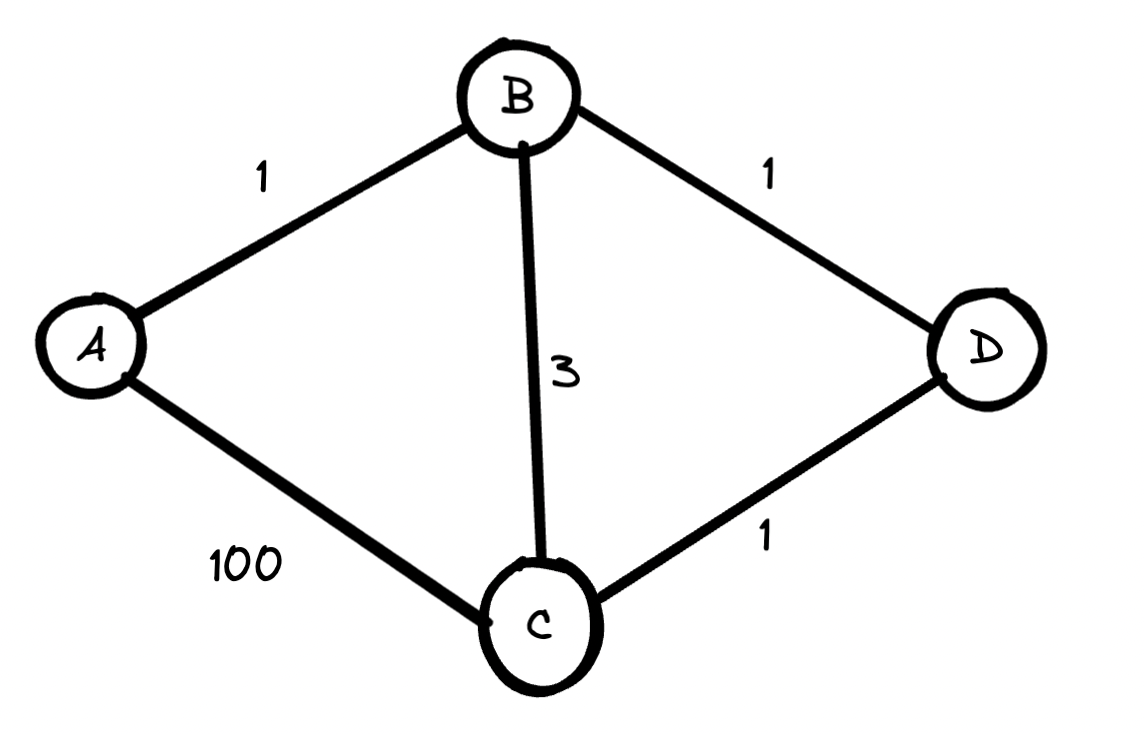
Answer: 3 (\(A \rightarrow B \rightarrow D \rightarrow C\)).
Correctness
Theorem 1 (Correctness of UCS): When a state \(s\) is popped from the frontier and moved to explored, its priority is \(PastCost(s)\), the minimum cost to \(s\). That is, once the state \(s\) is in explored, the cost is indeed the minimum.
For the proof, watch the video.
Interesting note: - We know that UCS cannot handle negatively-weighted edges. What happens if we just add some arbitrarly large constant to all edges to make them positive and then solve this. Will this work? - NO! See here. It penalizes longer paths more than shorter paths, so we would end up solving a different problem. Paths with more num edges are penalized more than less edges but more weight. If the original path was many small weight edges, but there also exists a large edge(s), the add constant scenario would penalize the many small weights much more and thus the minimum path can change.
DP vs. UCS
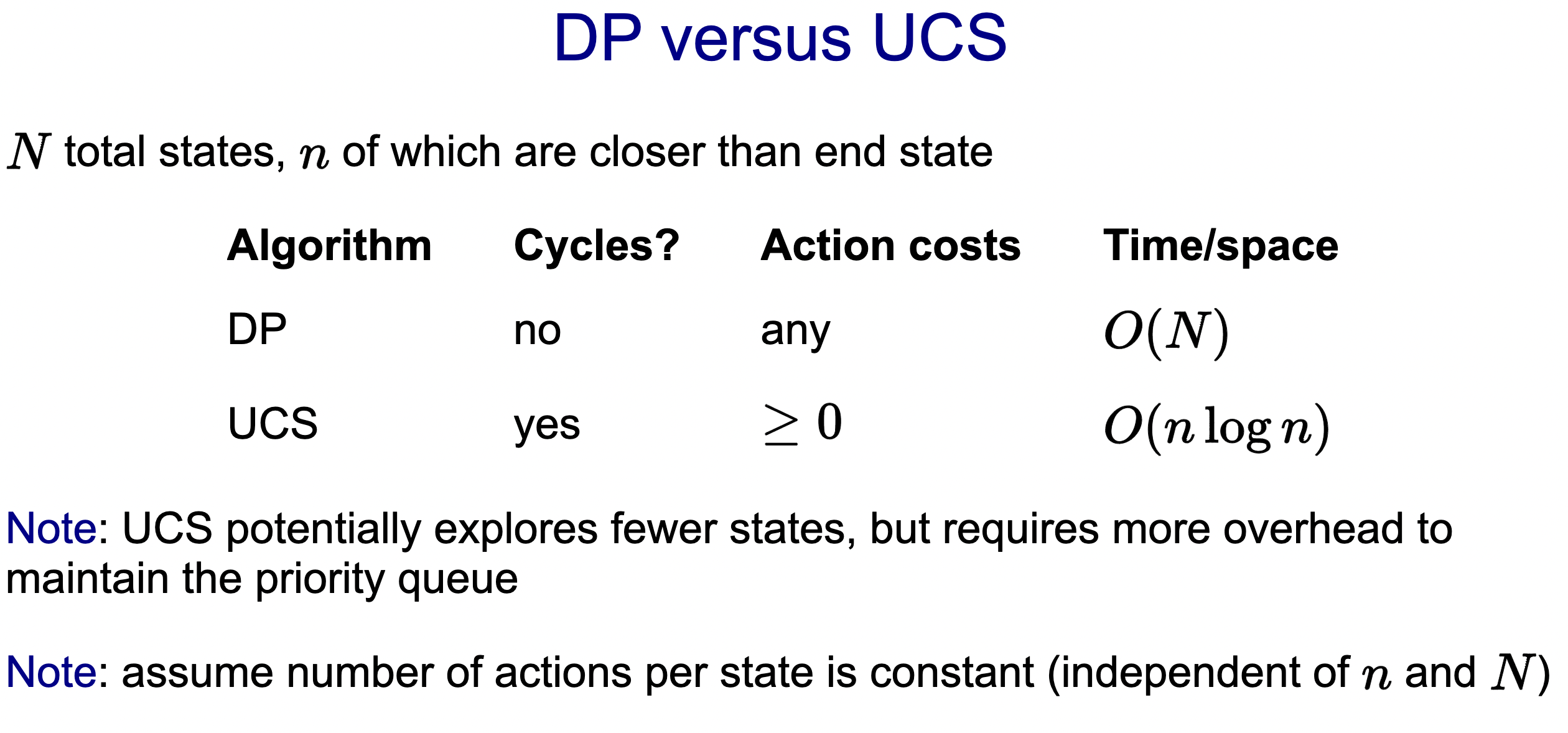
- DP can handle negative costs, UCS cannot.
- Because of the above, DP has to explore all \(N\) reachable states from the start state (inefficient). However, UCS can avoid this since their are no negative costs.
- On the contrary, UCS only needs to explore \(n\) states where \(n\) is the number of states such that each of these states are cheaper to get to than the end state.
- UCS can handle cycles. DP cannot.
- UCS has some additional overhead with handling the priority queue, in lookup time.
Summary thus far:
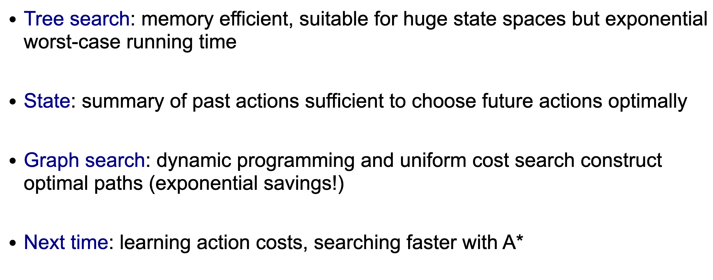
- We started out with the idea of a search problem, an abstraction that provides a clean interface between modeling and algorithms.
- Tree search algorithms are the simplest: just try exploring all possible states and actions. With backtracking search and DFS with iterative deepening, we can scale up to huge state spaces since the memory usage only depends on the number of actions in the solution path. Of course, these algorithms necessarily take exponential time in the worst case.
- To do better, we need to think more about bookkeeping. The most important concept from this lecture is the idea of a state, which contains all the information about the past to act optimally in the future. We saw several examples of traveling between cities under various constraints, where coming up with the proper minimal state required a deep understanding of search.
- With an appropriately defined state, we can apply either dynamic programming or UCS, which have complementary strengths. The former handles negative action costs and the latter handles cycles. Both require space proportional to the number of states, so we need to make sure that we did a good job with the modeling of the state.
A-star is next. But this algorithm is the same as UCS, except we calculate the cost differently. We use a heuristic to guide us towards the end goal better. A hueristic is just some function \(f(x)\) where \(x\) is a given state.