Week 2, Lecture 1 - Machine Learning III

Date: 10/5/22

Module: Generalization

Module: Best practices

Module: K-means

We will now go over a powerful unsupervised learning algorithm that divides the data into “clusters” based on similarity.

Idea:

• input: large amounts of raw text
• output: distinct clusters. e.g.,:
  • Cluster 1: Friday Monday Thursday…
  • Cluster 2: June March July April…
  • .
  • .
  • .
  • Cluster n: water gas coal liquid acid

As opposed to supervised learning, we don’t use labels in unsupervised learning (i.e., no supervision). The model learns the structure automatically. This is important since labels are difficult to obtain but it is often the case that unlabeled data is very easy to get an abundance of.

Here is the general idea of clustering:

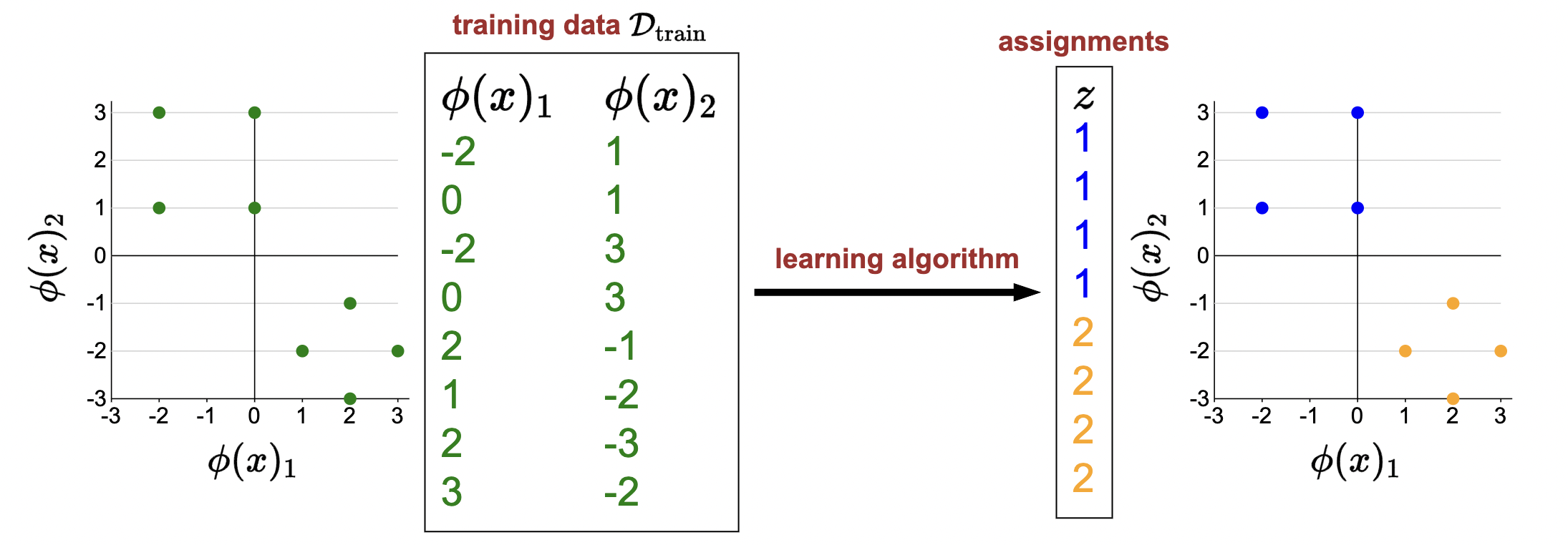
• Take in a bunch of unlabeled feature vectors
• Assign each datum to a “cluster”
• We define two clusters (1, blue; 2, orange).
• Datum, when plotted in euclidean space, should be assigned to nearby clusters.

Ok… let’s get a little more formal.

Clustering: the task

Note

Definition 1 (Clustering)

Input: training points \[ \mathcal{D}_{\text {train }}=\left[x_1, \ldots, x_n\right] \] Output: assignment of each point to a cluster \(\mathbf{z}=\left[z_1, \ldots, z_n\right]\) where \(z_i \in\{1, \ldots, K\}\)

¹

• We call \(\mathbf{z}=\left[z_1, \ldots, z_n\right]\) the assignment vector.
• Make sure to understand the above point: what we are outputting is a vector, of length \(n\) where \(n\) is the length of the dataset, where each \(i\)th component maps the \(i\)th data point to one of the \(z\) clusters (i.e., \(z_i \in\{1, \ldots, K\}\)).
  • That is, “For each \(i, z_i \in\{1, \ldots, K\}\) specifies which of the \(K\) clusters point \(i\) is assigned to.” (221).

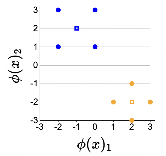
Centroids

Ok… what the hell is a cluster even? How do we define this mathematically. Well, a cluster is represented by a centroid.

Note

Definition 2 (centroid)

Each cluster \(k=1, \ldots, K\) is represented by a centroid \(\mu_k \in \mathbb{R}^d\).

\[\boldsymbol{\mu}=\left[\mu_1, \ldots, \mu_K\right]\]

each component in \(\boldsymbol{\mu}\) is a coordinate² representing the “center” of that cluster.

Visual (unfilled squares are the plotted centroids):

\(K\)-means objective

Now that we understand clustering and centroids, the intuition is easy to see.

Intuition: want each point \(\phi\left(x_i\right)\) to be close to its assigned centroid \(\mu_{z_i}\).

from this, we can develop the \(K\)-means objective (i.e., the loss).

Note

Definition 3 (\(K\)-means objective)

\[\operatorname{Loss}_{k m e a n s}(\mathbb{z}, \mu)=\sum_{i=1}^n\left\|\phi\left(x_i\right)-\mu_{z_i}\right\|^2\]

\[\min _{\mathrm{z}} \min _\mu \operatorname{Loss}_{\mathrm{kmeans}}(\mathrm{z}, \mu)\]

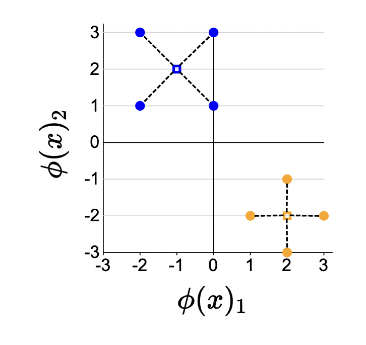
• In words, we are saying that, given an assignment vector for each of the data points (i.e., model prediction) and a centroid vector, minimize the squared distance between each in an element-wise (indexed) fashion.
• Note that \(\phi\left(x_i\right)-\mu_{z_i}\) is just measuring the distance between the input feature vector and the predicted centroid.
• We take this squared distance for each individual datum and then sum it up for the entire dataset to define the \(K\)-means objective.

Algorithm intuition

Before we introduce the algorithm to solve this objective, let’s go over some intuition with a 1d example consisting of 4 data points.

The idea is pictorially displayed as follows:

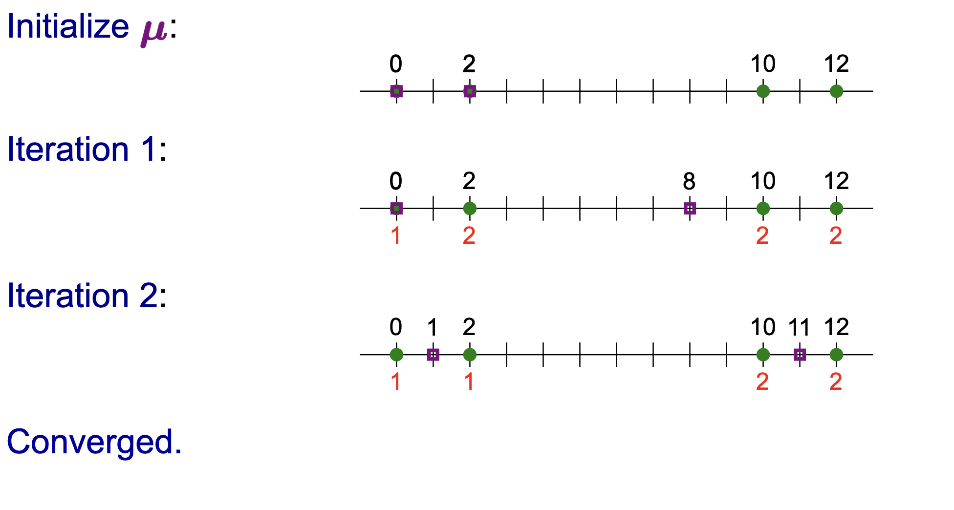
• We start off by knowing nothing: no known assignments or centroids. Intuitively, we choose that we need \(2\) clusters (I think we must choose the number of clusters beforehand).
• We randomly initialize the coordinates for the two centroids representing the two clusters.
• We run one iteration of an algorithm… repeat until convergence.

(expand on this)

Ok… so what is the juicy details behind this magical algorithm. Before we mathematically introduce it, here is the general idea:

Note

We can think of the loss/objective as a reconstructive loss: as we iterate, we update our assignments and centroids at once. How do we update these? At each step, alternate between choosing the best assignments given the centroids, and choosing the best centroids given the assignments.

Notice that only the centroids are moved (the feature vectors don’t move but the assignment vector \(\mathbf{z}\) changes).

Ok… onto the actual algorithm.

\(K\)-means algorithm

Note

Definition 4 (\(K\)-means algorithm)

Our goal is to continiously update our assignments (\(\mathbf{z}\)) and centroids (\(\boldsymbol{\mu}\)).

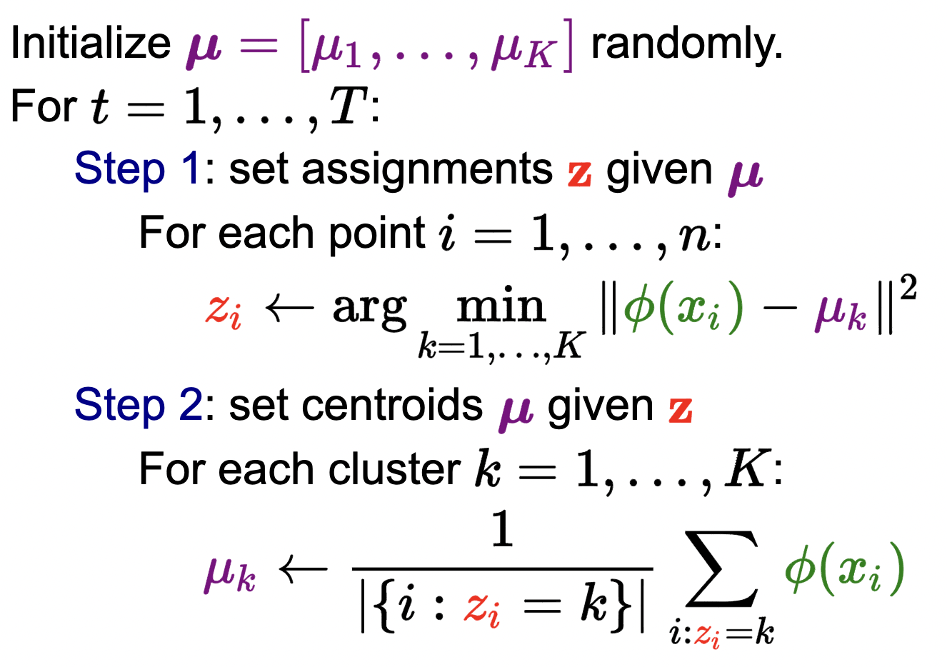
In words:

• Start by initializing all the centroids randomly. Then, we iteratively alternate back and forth between steps 1 and 2, optimizing \(\mathbf{z}\) given \(\mathbf{\mu}\) and \(\mathbf{\mu}\) given \(\mathbf{z}\) ³.
• Step 1 (update \(\mathbf{z}\)): at this time, we care about assigning the best centroid to each data point. This is straightforward: just assign the one that is closest to it, squared distance-wise. We hold the centroids in place and don’t change them here.
  • That is, the best label for \(z_i\) is the cluster \(k\) that minimizes the distance to the centroid \(\mu_k\).
  • Formally, we are optimizing the \(K\)-means objective with respect to the assignment vector \(\mathbf{z}\).
• Step 2 (update \(\mathbf{\mu}\)): turns things around: let’s hold the assignments (\(\mathbf{z}\)) in place and choose the best centroids given these assignments. We do this via the \(K\)-means objective and optimize it with respect to the centroids \(\mathbf{\mu}\).
  • In English, we place the centroid \(\mu_k\) at the average of all the points assigned to cluster \(k\).
• of K-means fixes the centroids . Then we can optimize the K-means objective with respect to alone quite easily. It is easy to show that the best label for is the cluster that minimizes the distance to the centroid (which is fixed). Step 2 turns things around and fixes the assignments . We can again look at the K-means objective function and optimize it with respect to the centroids . The best is to place the centroid at the average of all the points assigned to cluster .

• Note on minima:
  • tl;dr \(K\)-means is guaranteed to converge to a local minimum (i.e., loss is gaurenteed to decrease at each iteration), but is not guaranteed to find the global minimum. Run multiple times from different random initializations such that you don’t keep on getting stuck at a local minimum.
  • K-means is guaranteed to decrease the loss function each iteration and will converge to a local minimum, but it is not guaranteed to find the global minimum, so one must exercise caution when applying K-means.
  • Advanced: One solution is to simply run K-means several times from multiple random initializations and then choose the solution that has the lowest loss.
  • Advanced: Or we could try to be smarter in how we initialize K-means. K-means++ is an initialization scheme which places centroids on training points so that these centroids tend to be distant from one another.

Footnotes

1. lingering question: do we define how many clusters there are and where they lie explicity? Or is this learned automatically?

2. realize that this component must be of the same dimension and space of the input feature vectors. See the visual to understand why.

3. do we do steps 1 and 2 for each iteration or alternate?