Week 2, Lecture 1 - Machine Learning II
Date: 10/3/22
Module: Group DRO
“How to ensure more equitable performance.”
- Motivation:
- Thus far, our goal has been to minimize training loss with the hope that our model will perform well on new examples.
- However, train loss is defined as the average of all individual losses on each sample.
- Equally weighting every sample loss can lead to problems with equity.
- For example, unrepresented groups in the training data will have less representation in the loss and therefore in the model.
- group distributional robust optimization (group DRO) can help mitigate some of these inequalities.
- tl;dr: averaging training losses can lead to inequalities across groups, group DRO can help mitigate this.
- Example:
- Gender Shades project by Joy Buolamwini and Timnit Gebru discovered that Microsoft, Face++, and IBM’s gender classification system performed worse on darker-skinned females, while lighter-skinned data samples got nearly 100% accuracy.
- i.e., discrimination can arise from ML
- Has real life consequences: “Robert Julian-Borchak Williams was wrongly arrested due to a incorrect match with another Black man captured from a surveillance video, and this mistake was made by a facial recognition system”.
- Gender Shades project by Joy Buolamwini and Timnit Gebru discovered that Microsoft, Face++, and IBM’s gender classification system performed worse on darker-skinned females, while lighter-skinned data samples got nearly 100% accuracy.
How can we help mitigate this algorithmically?
Linear regression the standard way
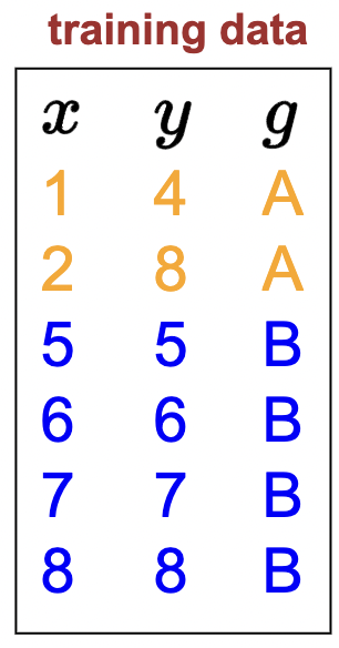
Take the following dataset, where each sample now as an addtional meta-datum: a group (e.g., some demographic).
Let’s setup the same model we used in last lecture’s linear regression module:
\[ f_{\mathbf{w}}(x)=\mathbf{w} \cdot \phi(x) \quad \mathbf{w}=[w] \quad \phi(x)=[x] \]
Important note: we don’t use (i.e., the predictor \(f_{\mathbf{w}}\)) does not use group information \(g\) to make a prediction.
And since this is linear regression, all models will be a line that passes through the origin, differing in the slope \(w\). Here is a plot of the training samples with the identity line:
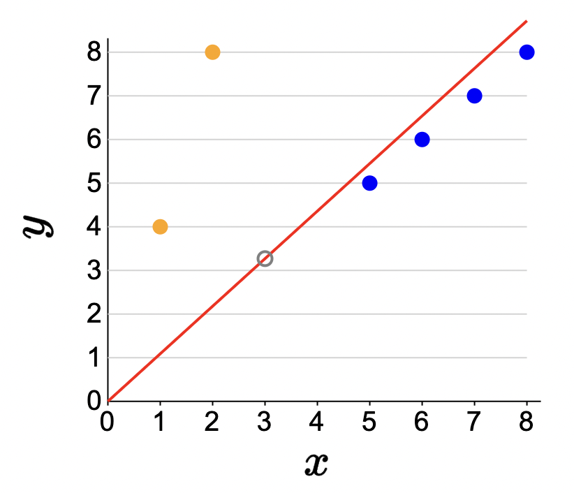
As we can see, certain values for \(w\) will be more beneficial for the blue group than the orange group. There is a bit of tension.
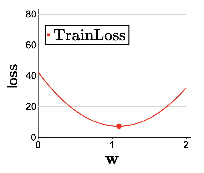
The classic way to solve a linear regression problem here is to minimize the train loss which is an average over all sample losses:
\[ min \operatorname{TrainLoss}(\mathbf{w})=\frac{1}{\left|\mathcal{D}_{\text {train }}\right|} \sum_{(x, y) \in \mathcal{D}_{\text {train }}} \operatorname{Loss}(x, y, \mathbf{w}) \]
with the above data points (and \(\operatorname{Loss}(x, y, \mathbf{w})=\left(f_{\mathbf{w}}(x)-y\right)^2\)), we have:
\[ \operatorname{TrainLoss}(1)=\frac{1}{6}\left((1-4)^2+(2-8)^2+(5-5)^2+(6-6)^2+(7-7)^2+(8-8)^2\right)=7.5. \]
doing some calculations, we see that \(\mathbf{w}=1.09\) produces the minimum train loss:
Using groups
Ok… let’s change one thing up (loss!) a couple of times.
Let’s calculate the loss for each group separately.
Per-group loss
From above, we define the train loss for some general group \(g\) as
\[ \operatorname{TrainLoss}_g(\mathbf{w})=\frac{1}{\left|\mathcal{D}_{\text {train }}(g)\right|} \sum_{(x, y) \in \mathcal{D}_{\text {train }}(g)} \operatorname{Loss}(x, y, \mathbf{w}). \]
plugging in for the above dataset:
\[\operatorname{TrainLoss}_{\mathrm{A}}(1)=\frac{1}{2}\left((1-4)^2+(2-8)^2\right)=22.5\]
\[\operatorname{TrainLoss}_{\mathrm{B}}(1)=\frac{1}{4}\left((5-5)^2+(6-6)^2+(7-7)^2+(8-8)^2\right)=0\]
Conclusion: huge performance drop-off from 0 to 22.5 loss for the underrepresented group (A). So, although the average loss is 7.5, we see the disparity for ourselves here. Many people won’t go this deep and assume their “7.5” loss is good enough.
Also, check this out:
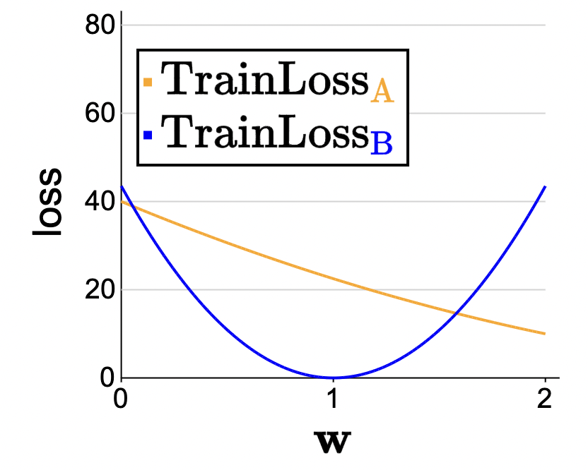
see how the minimum for group A and group B mean picking different values for \(\mathbf{w}\). But of course, we can only pick one \(\mathbf{w}\). Tension, tension!
Ok cool… but usually it is helpful to have just one value for the loss. I agree:
Maximum group loss
We can literally just perform per-group losses and just take the max of all of them (i.e., the worst case):
\[ \operatorname{TrainLoss}_{\max }(\mathbf{w})=\max _g \operatorname{TrainLoss}_g(\mathbf{w}). \]
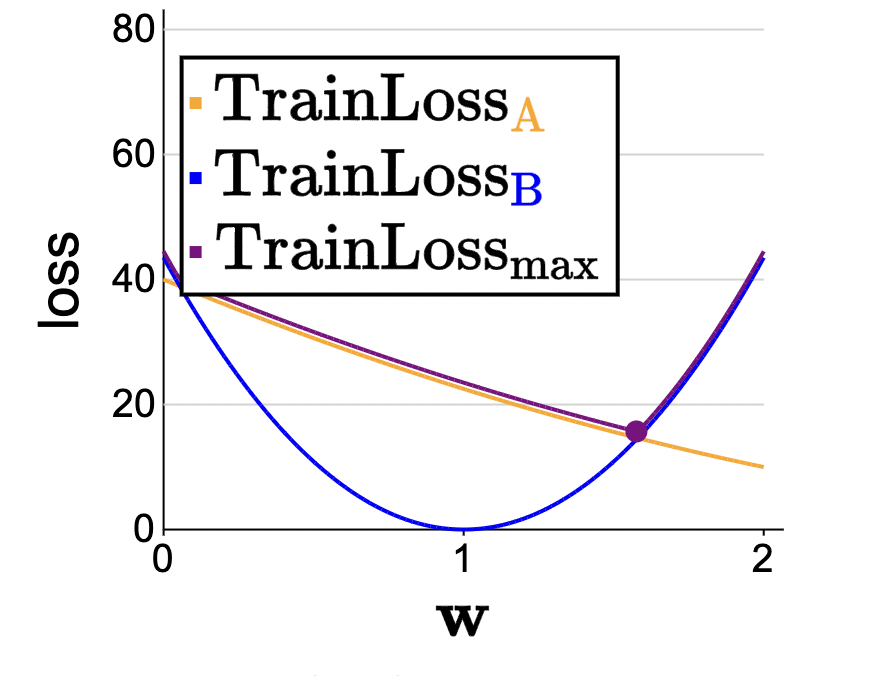
This function is the pointwise maximum of the per-group losses, which you can see on the plot as taking the upper envelope of the two per-group losses (cs 221).
We call this group distributionally robust optimization.
Average vs. group DRO
Alright… here are the results:
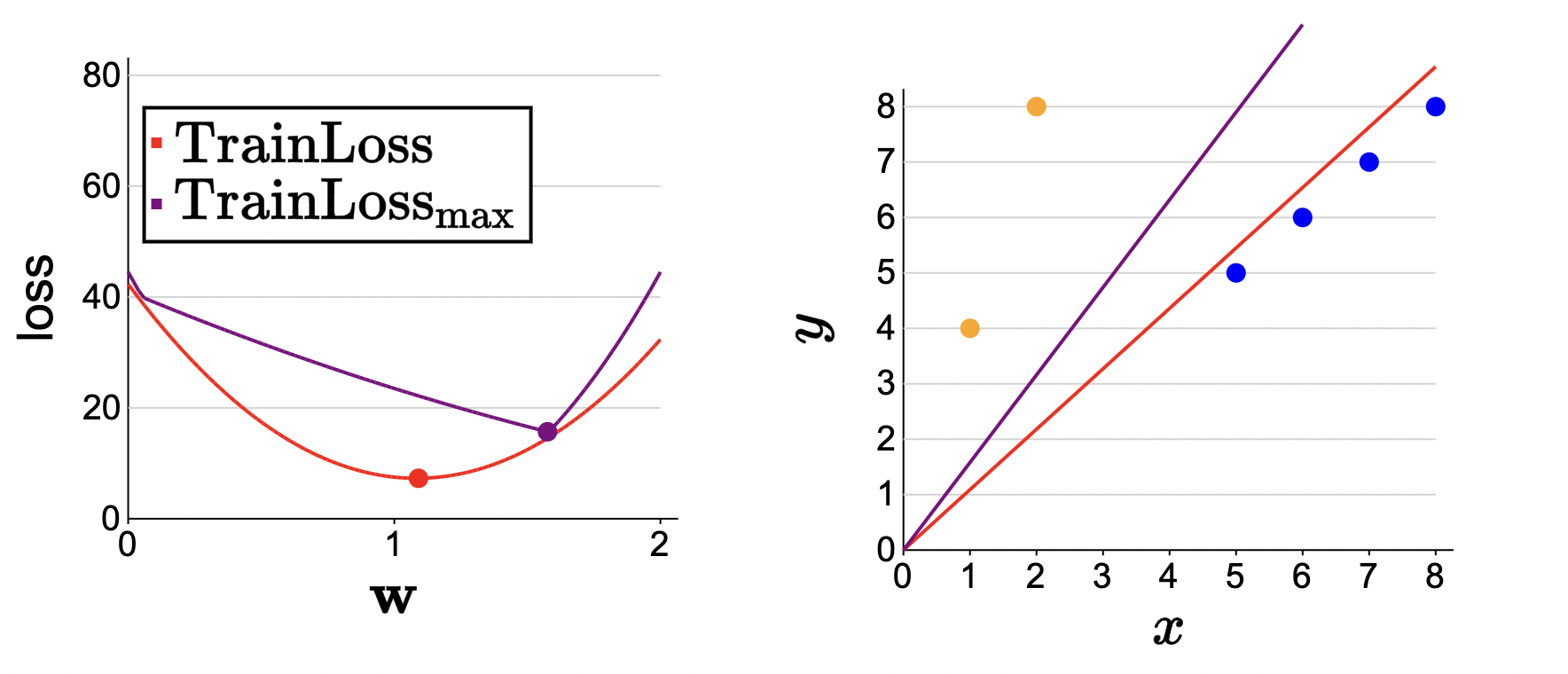
Here, a weight vector \(\mathbf{w}=1.09\) minimizes the loss for the average (traditional) case. However, using group DRO, we get \(\mathbf{w}=1.58\). So using \(\mathbf{w}=1.58\) might produce worse results but should be more equitable (see the learned purple line vs. the learning red line).
“Intuitively, the average loss favors majority groups over minority groups, but the maximum group loss gives a stronger voice to the minority groups, and as we see here, their influence is felt to a greater extent.” - CS 221.
Note on gradient descent
From the 221 slides:
- In general, we can minimize the maximum group loss by gradient descent, as usual.
- We just have to be able to take the gradient of TrainLoss \(_{\max }\) , which is a maximum over the per-group losses.
- The gradient of a max is simply the gradient of the term that achieves the max.
- So algorithmically, it’s very intuitive: you first compute whichever group (\(g^*\)) has the highest loss, and then you just evaluate the gradient only on per-group loss of that group (\(g^*\)).
In math:
\[ \begin{aligned} &\operatorname{TrainLoss}_{\max }(\mathbf{w})=\max _g \operatorname{TrainLoss}_g(\mathbf{w}) \\ &\nabla \operatorname{TrainLoss}_{\max }(\mathbf{w})=\nabla \operatorname{TrainLoss} g_{g^*}(\mathbf{w}) \\ &\text { where } g^*=\arg \max _g \operatorname{TrainLoss}_g(\mathbf{w}) \end{aligned}. \]
Note that SGD cannot be applied in vanilla form since its not an average, it is a max of an average1.
Some other notes to consider: - When we have multiple attributes (gender, race), intersectionality becomes difficult to incorporate. - For further reading, consider checking out the book Fairness and machine learning: Limitations and Opportunities, and a paper that explores group DRO for neural networks.
Module: Non-linear features (offline)
How to get non-linear functions from linear machinery.
- Linear regression/classification: fit some straight line to some data: \(\mathcal{F}=\left\{f_{\mathbf{w}}(x)=\mathbf{w} \cdot \phi(x): \mathbf{w} \in \mathbb{R}^d\right\}\).
- Recall hypothesis class: what are the possible predictors that the learning algorithm can consider?
- Works well for linear data.
However… not all data is linear:
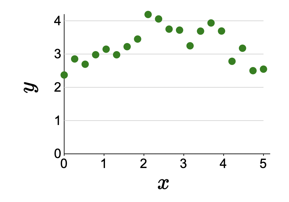
how can we fit a non-linear predictor to generalize for this data?
Quadratic predictors
- Change the feature extractor to include non-linear components/features. Example:
\[\phi(x)=\left[1, x, x^2\right].\]
Example: \(\phi(3)=[1,3,9]\). With some various weight combinations, we’d get something like:
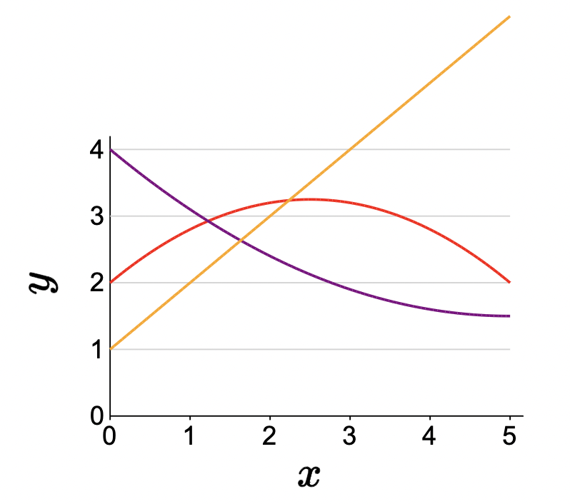
- Note that by setting the weight for feature \(x^2\) to zero, we recover linear predictors.
- Here, the hypothesis class is the set of all predictors \(f_{\mathbf{w}}\) obtained by varying \(\mathbf{w}\).
Piecewise constant predictors
- Quadratic only can fit smooth and linear curves. But we…
- Can carry on this idea to other math forms to better capture the input space.
- Piecewise: expressive non-linear predictors by partitioning the input space.
\[ \phi(x)=[\mathbf{1}[0<x \leq 1], \mathbf{1}[1<x \leq 2], \mathbf{1}[2<x \leq 3], \mathbf{1}[3<x \leq 4], \mathbf{1}[4<x \leq 5]] \]
Example: \(\phi(2.3)=[0,0,1,0,0]\). Visual with:
\[f(x)=[1,2,4,4,3] \cdot \phi(x)\] \[f(x)=[4,3,3,2,1.5] \cdot \phi(x)\] \[\mathcal{F}=\left\{f_{\mathbf{w}}(x)=\mathbf{w} \cdot \phi(x): \mathbf{w} \in \mathbb{R}^5\right\}\]
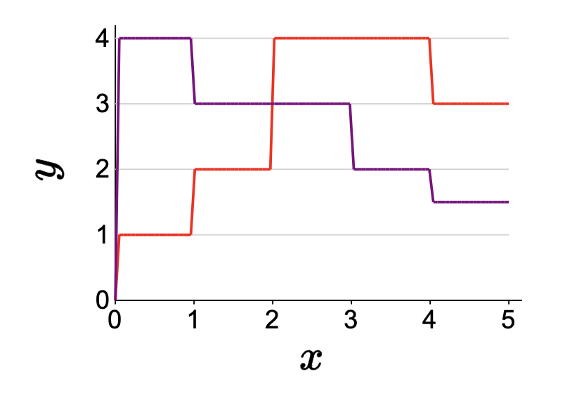
- Each component of the feature vector corresponds to one region and is 1 if \(x\) lies in that region and \(0\) otherwise.
- Predicted value is just the weight.
- Can make regions smaller. In the limit, we’d be able to capture any predictor we want.
- But if the input is multi-dimensional (\(d\)), then we’d have \(B^{d}\) features where \(B\) is number of bins.
Periodic predictors
- Add in a trigonometric function in the feature extractor.
\[\phi(x)=\left[1, x, x^2, \cos (3 x)\right]\]
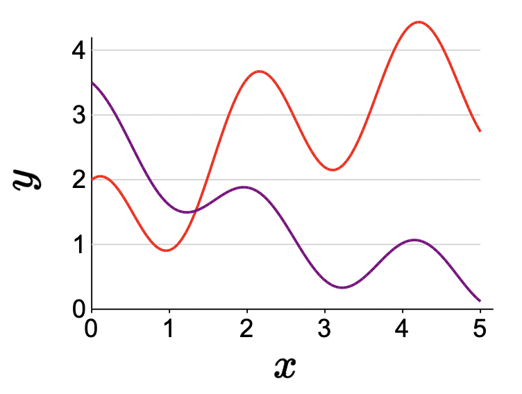
The general idea
- Key idea has been to incorporate a non-linear math function in the feature extractor.
- Generally, the choice of features is informed by the prediction task that we wish to solve
- For example, if \(x\) represents time and we believe the true output \(y\) varies according to some periodic structure, we can incorporate a periodic feature in the feature extractor.
- Features represent what properties might be useful for prediction. If a feature is not useful, then the learning algorithm can assign a weight close to zero to that feature. Of course, the more features one has, the harder learning becomes.
Note:
- We still have a linear classifier as the simple dot product \(\mathbf{w} \cdot \phi(x)\) is indeed linear in \(\mathbf{w}\) and \(\phi(x)\). However, the feature extractor components can mean that we aren’t linear in just \(x\).
- The significance is that we can acheive non-linearity through the FE but the learning optimizer/algorithm thinks we just have a linear predictor (so optimizing the weights is still efficient!)
Aside (convexity): if the score (logit) is linear in just \(\mathbf{W}\) (i.e., \(\mathbf{W}\) is a linear vector (as it usually is as its just scalar numbers) and \(\texttt{Loss}\) is convex, then gradient descent is gaurenteed to converge to a global minimum.)
Definition 1 (Non-linearity):
- Expressivity: score w \(\boldsymbol{\phi}(\boldsymbol{x})\) can be a non-linear function of \(x\)
- Efficiency: score \(\mathbf{w} \cdot \phi(x)\) always a linear function of \(\mathbf{w}\)
Classifiers
- Regression to classification: instead of using the predictor curve (decision boundary) to predict \(y\) from new \(x\)’s, let’s use the curve to classify \(x\) and
positiveornegative(corresponding to the sides of the decision boundary). Recall \(f_{\mathbf{w}}(x)=\operatorname{sign}(\mathbf{w} \cdot \phi(x))\). - Non-linearity arises here then in that we can make the decision curve non-linear.
From this:
to this:
how? Introduce non-linear functions in feature extractor:
\[\phi(x)=\left[x_1, x_2, x_1^2+x_2^2\right],\] \[f(x)=\operatorname{sign}([2,2,-1] \cdot \phi(x))\] or equivalently: \[ f(x)= \begin{cases}1 & \text { if }\left(x_1-1\right)^2+\left(x_2-1\right)^2 \leq 2 \\ -1 & \text { otherwise }\end{cases} \]
See this awesome video animation for understanding how we can still have a linearity in \(\phi(x)\) but non-linearity in \(x\). Idea is that the raw \(x\) isn’t linearly seperable, but we can project the raw \(x\) into some different dimension (i.e., adding a feature changes the dimension of the vector) non-linearly (e.g., onto a polynomial in \(\mathbf{R}^{n + 1}\)) which we can then have a linear hyperplane as the decision boundary (how SVMs work!).
Question: how can we generalize a decision boundary for \(n\)-way classification for \(n > 2\)? Answer: create \(n\) binary classifiers!
Module: Feature templates (offline)
How to design and organize features.
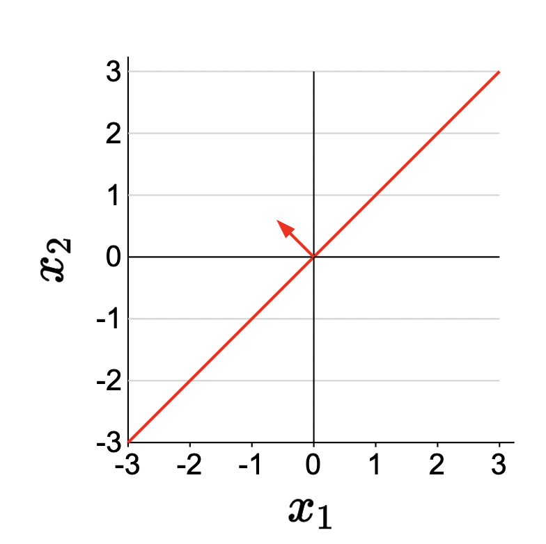
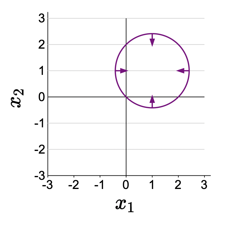
Motivation: hypothesis class is too big because we let \(\mathbf{w}\) vary freely.
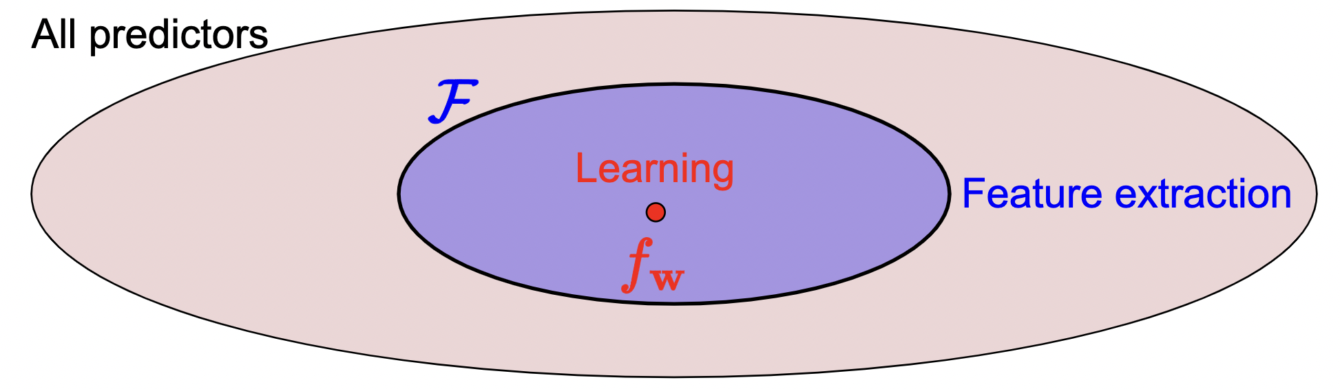
We can narrow this down to the smaller circle by using a feature extractor. Then, choose \(f_{\mathrm{w}} \in \mathcal{F}\) based on data. So how do we narrow this down and choose a good feature extractor?
In \(\mathbf{w} \cdot \phi(x)\), the weight corresponds to the magnitude of importance for the corresponding feature extraction component. The polarity is also assigned.
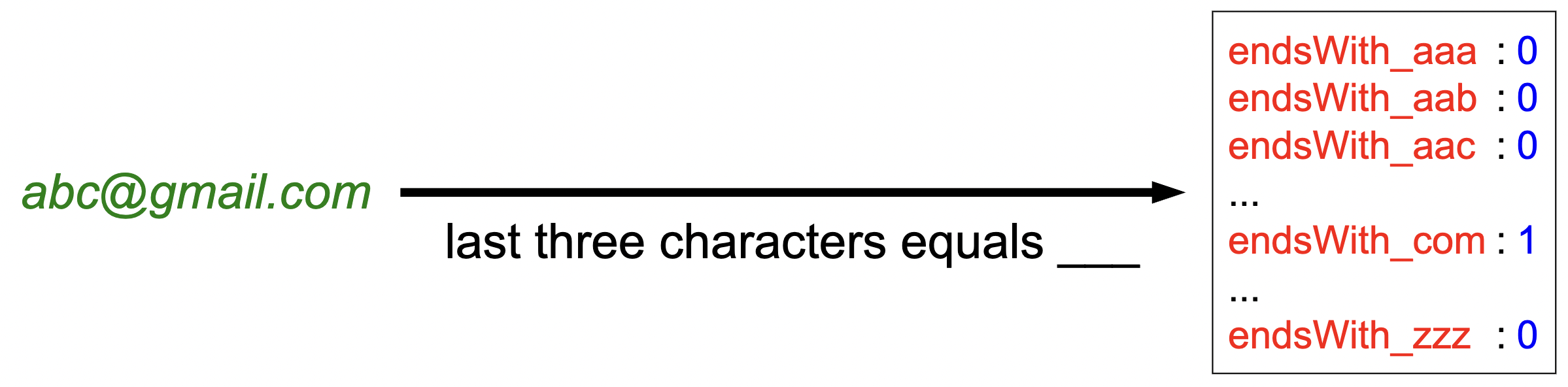
Definition 2 (Feature template): A feature template is a group of features all computed in a similar way.
Example: say we have this task:

given an input string, determine if this is a valid email address. We can try to hand-construct features such as “contains @”. But this isn’t a general framework. So instead, we can define feature templates where we say something like
- Template: “last three characters equals _ _ _”
- Resultant features:
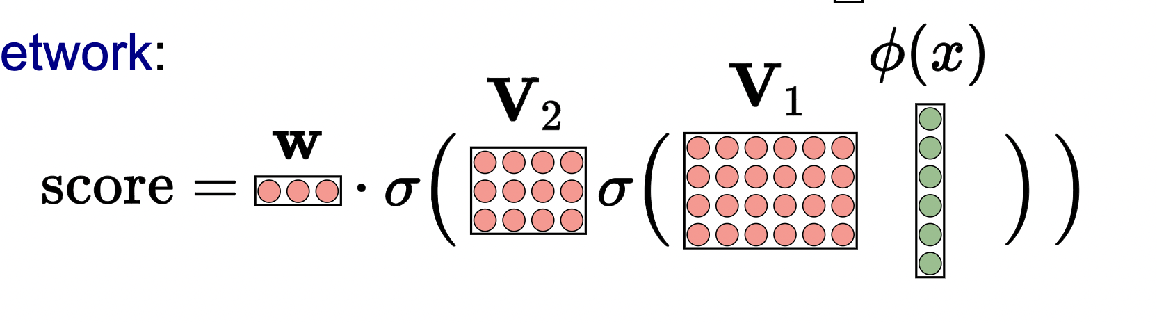
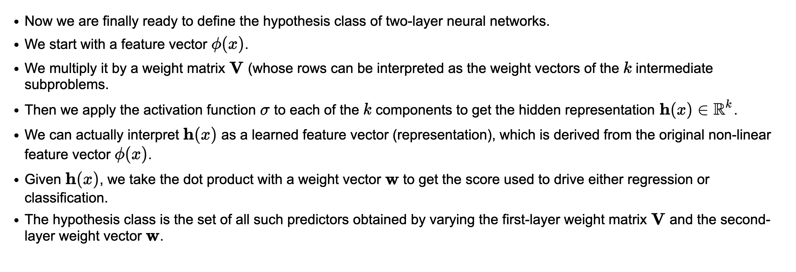
Module: Neural networks
- In summary, acheive end-to-end non-linearity without needing to define a feature extractor.
- Screw hand-configuring the feature extractor \(\phi(x)\). Throw this away. Then, define activation functions that take in the logits from each dot product. That is how we acheive non-linearity. And guess what?!: this is implicitly learned in gradient descent (why though?)!
- Then, stack a bunch of these on top of each other to get a deep NN!
Notes:
- Can achieve non-linear classifier with feature extraction manipulation too. But…
- Have to hand-learn features
- as \(d\), dimension of vector increases, we need \(O\left(d^2\right)\) features. Computationally hard.
- neural networks yield non-linear predictors in a more compact way.
- Activation function avoids zero-gradients.
Helpful slide:
Module: Backpropagation
Computation graphs and backpropagation algorithm for computing gradients to optimize the weights of neural networks.
- For each time we want to update our weights in a neural network, we have to do so weight respect to each weight vector in the weight matrix. This wasn’t a problem for linear predictors because the gradient only deals with one parameter weight vector. Neural nets have many params we need to tune and calculate gradients with respect too!
\[\operatorname{Loss}\left(x, y, \mathbf{V}_1, \mathbf{V}_2, \mathbf{V}_3, \mathbf{w}\right)=\left(\mathbf{w} \cdot \sigma\left(\mathbb{V}_3 \sigma\left(\mathbb{V}_2 \sigma\left(\mathbb{V}_1 \phi(x)\right)\right)\right)-y\right)^2,\]
\[ \begin{aligned} &\mathbf{V}_1 \leftarrow \mathbf{V}_1-\eta \nabla_{\mathbf{V}_1} \operatorname{Loss}\left(x, y, \mathbf{V}_1, \mathbf{V}_2, \mathbf{V}_3, \mathbf{w}\right) \\ &\mathbf{V}_2 \leftarrow \mathbf{V}_2-\eta \nabla_{\mathbf{V}_2} \operatorname{Loss}\left(x, y, \mathbf{V}_1, \mathbf{V}_2, \mathbf{V}_3, \mathbf{w}\right) \\ &\mathbf{V}_3 \leftarrow \mathbf{V}_3-\eta \nabla_{\mathbf{V}_3} \operatorname{Loss}\left(x, y, \mathbf{V}_1, \mathbf{V}_2, \mathbf{V}_3, \mathbf{w}\right) \\ &\mathbf{w} \leftarrow \mathbf{w}-\eta \nabla_{\mathbf{w}} \operatorname{Loss}\left(x, y, \mathbf{V}_1, \mathbf{V}_2, \mathbf{V}_3, \mathbf{w}\right) \end{aligned} \]
- This is tedious and expensive. Instead, we can create a computation graph and see the relaton between gradients. This is the main idea behind the backpropogation algorithm.
- We harness the idea that the gradients of e.g., \(\mathbf{V}_3\) depend on \(\mathbf{V}_2\) and \(\mathbf{V}_1\) gradients.
Definition 3 (Computation graph): A directed acyclic graph whose root node represents the final mathematical expression and each node represents intermediate subexpressions.
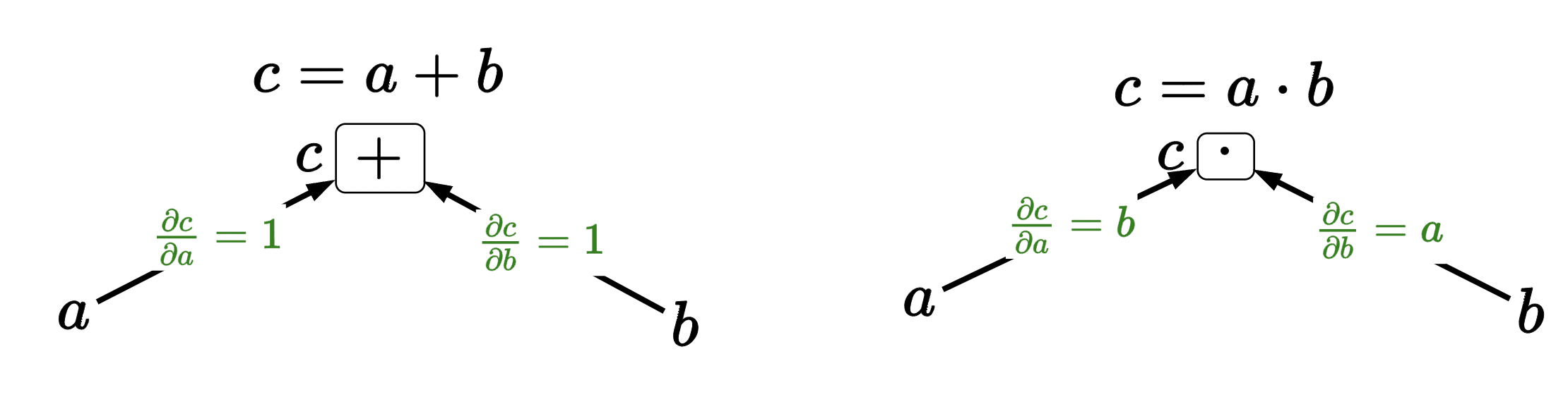
Functions as boxes
The main idea is to think of functions as boxes and calculate the gradient upwards with respect to each leave node. Example:
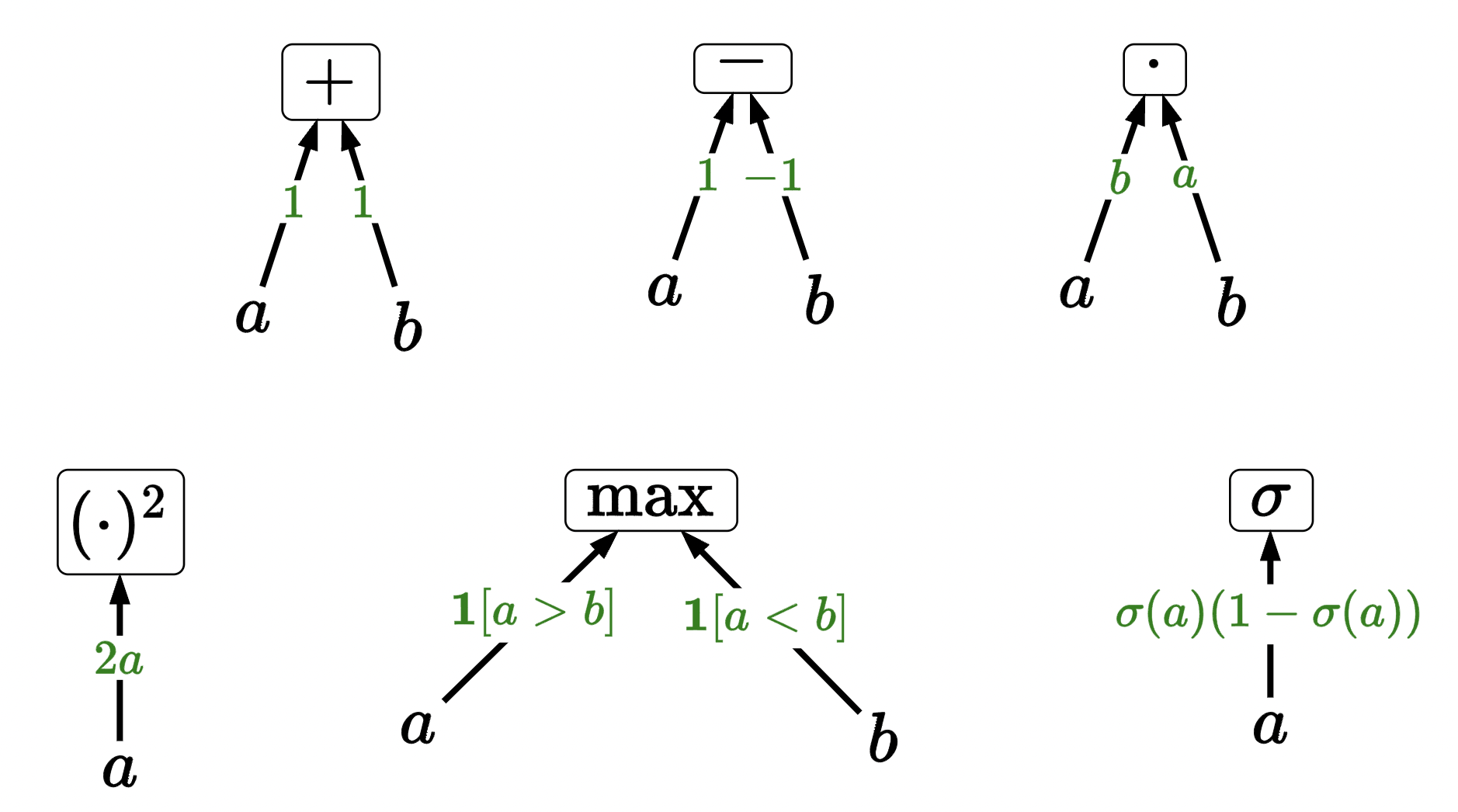
we can define these for some basic, common functions (basic building blocks):
we can now compose these building blocks to make more complicated functions. Example:
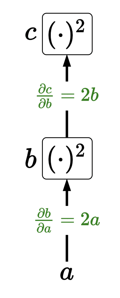
by chain rule (note \(b=a^2\)), we have \(\frac{\partial c}{\partial a}=\frac{\partial c}{\partial b} \frac{\partial b}{\partial a}=(2 b)(2 a)=\left(2 a^2\right)(2 a)=4 a^3\). To obtain complete gradient, multiply up the graph. We can also hash into specific points to get the individual gradients with respect to the successor node (which is exactly what we need for autodiff’ing neural nets! because we can get gradients with respect to \(\mathbf{V}_3\), \(\mathbf{V}_2\), \(\mathbf{V}_1\) just by hashing into a dict instead of re-calculating (kinda like memoization!)).