Week 1, Lecture 2 - Machine Learning I
Date: 9/28/22
Module: Overview
We now begin our journey into ML. Next 3 lectures. Reflex-based models to logic.
Reflex-based models
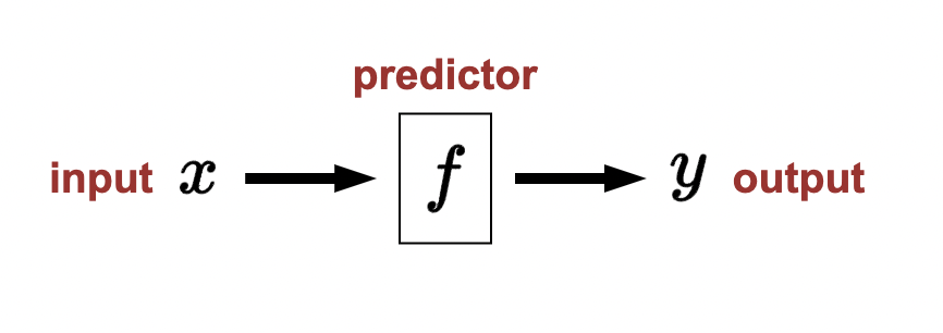
- Reflex-based models: a predictor \(f\) takes some input \(x\) and produces some output \(y\).
- Input can usually be anything but output is usually restricted (output defines the task).
First examples:
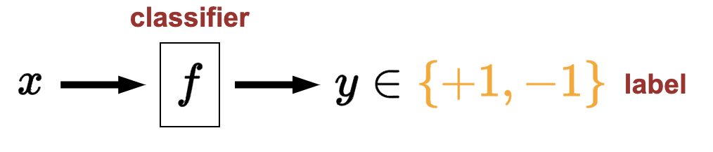
- Binary classifier: restrict \(y\): \(x \longrightarrow f \rightarrow y \in\{+1,-1\} \text { label }\).
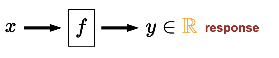
- Regression: \(x \longrightarrow f \rightarrow y \in \mathbb{R} \text { response }\).
- Arbitrary input with output restricted to some real number.
- Infinite continuous (whereas classification is finite discrete)
- Output is called the response: \(y \in \mathbb{R}\).
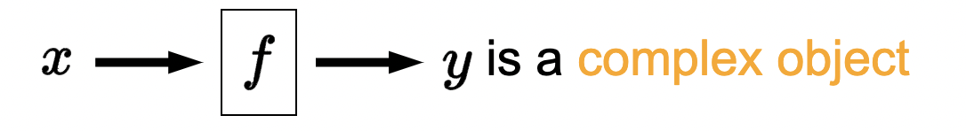
- Structured prediction: catch-all generalization for non-categoricalizable machine learning problems.
- e.g., image segmentation. Most tasks reduce to series of multi-class categorization problems. For example, image segmentation reduces to \(m \times n\) multi-class (or binary) classification problems where \(m, n\) are the dimensions of the image in pixels.
Roadmap
- Tasks:
- classification
- regression
- Algorithms:
- SGD
- backpropogation
- Models:
- non-linear features
- feature templates
- neural networks
- differentiable programming
- Misc. considerations:
- Group DRO (unbiasing objectives)
- Generalization
Module: linear regression
History: Ceres (asteroid) went behind the sun and scientists wanted to know when it would be observed again. Using data points gathered before it went behind the sun, Gauss used linear algebra to invent least squares linear regression to solve this task.
General framework:
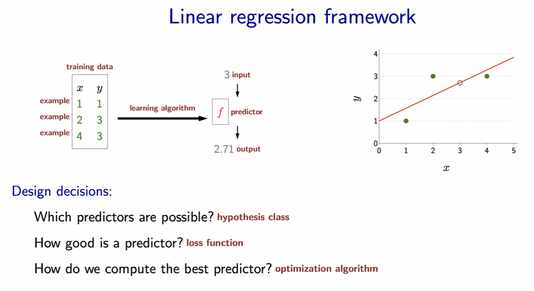
- Hypothesis class: which predictors (i.e. models) are possible?
- Linear, quadratic, neural network, etc. These all belong to the hypothesis class of the process.
- How good is predictor: loss function
- How to compute best fit curve: optimization algorithm
- Though looping through all possible predictors is computationally impossible so we use optimization to numerically approximate best fit curve. 1
Modeling
Definition 1 Hypothesis class: When we say hypothesis class, we mean the range of predictors that we can learn. For example, linear classifiers are of the form \(f(x)=w_1+w_2 x\) for some \(w_1\) and \(w_2\):
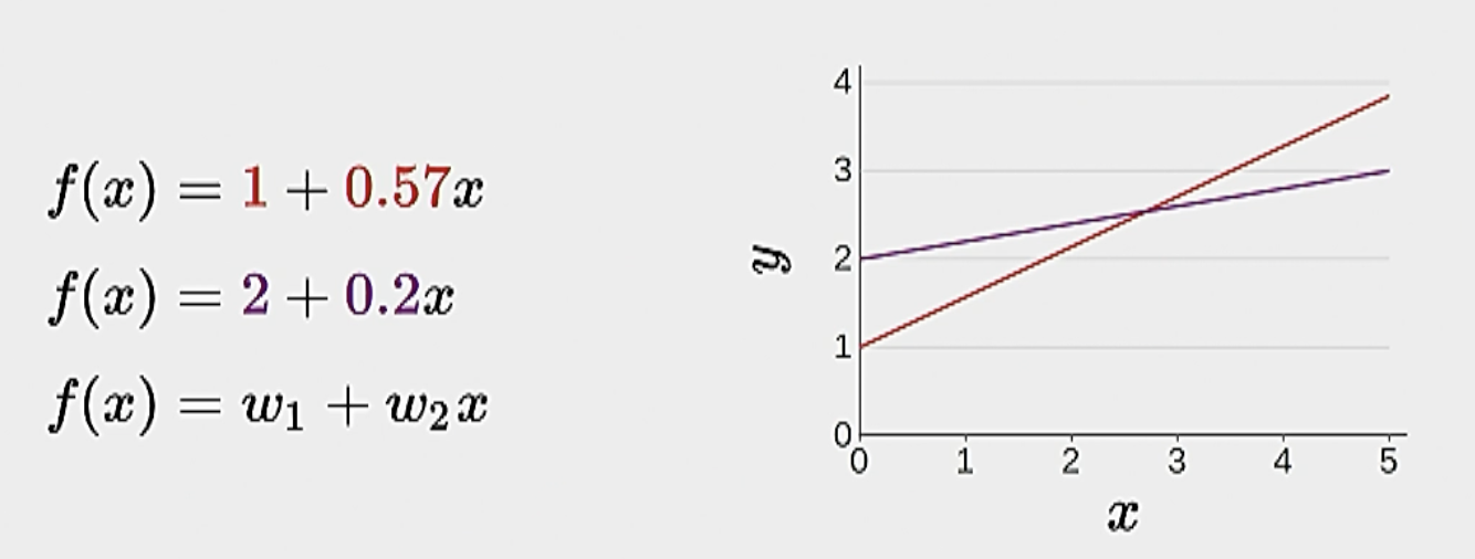
- This is cool and all, but if we want to add complexity, we should keep our notation simple. So here we will introduce the above with vector notation.
Definition 2 Vector notation for linear regression:
Weight vector: \[ \mathbf{w}=\left[w_1, w_2\right] \]
Feature extractor:
\[ \phi(x)=[1, x] \]
Takes in input vector \(x\) and returns transformed version of \(x\) to be fed into the model. We do this such that the input can be of the proper shape for the matrix multiplication that is to come or just oe extract general features that might lead to better performance. - Prediction (score):
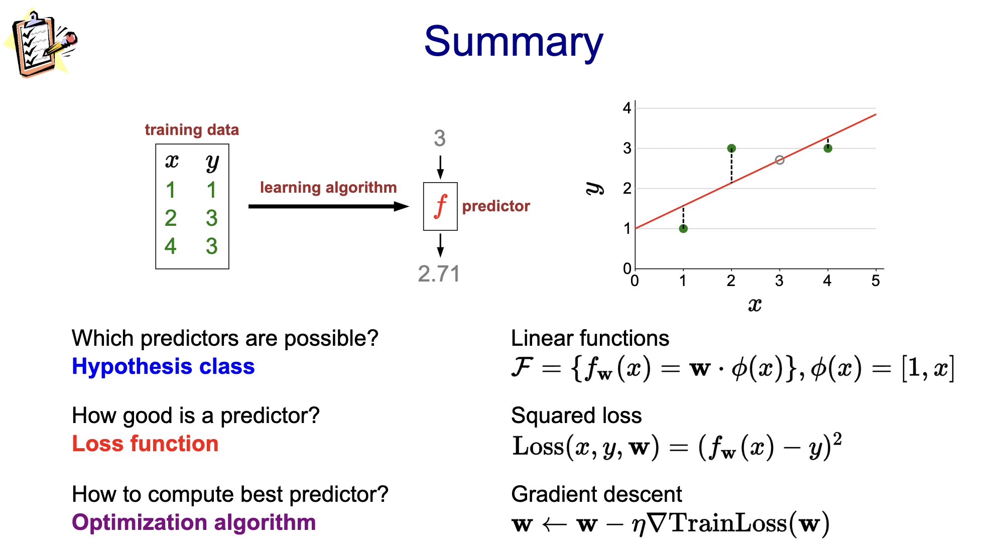
\[ f_{\mathbf{w}}(x)=\mathbf{w} \cdot \phi(x) \]
Example: \(f_{\mathbf{w}}(3)=[1,0.57] \cdot[1,3]=2.71\). Hypothesis class: \(\mathcal{F}=\left\{f_{\mathbf{w}}: \mathbf{w} \in \mathbb{R}^2\right\}\). i.e., a set of weight real-valued functions.
Next let’s move onto the loss function.
Loss function
- How good is a predictor? Here we “define” good.
- Example: least residual squares:
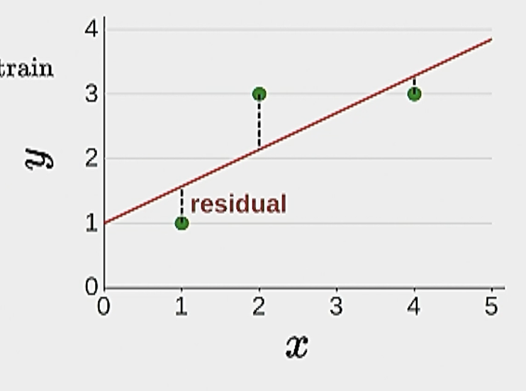
\[\operatorname{Loss}(x, y, \mathbf{w})=\left(f_{\mathbf{w}}(x)-y\right)^2\]
The above equation defines the loss for one data point. During training, we’d average all of the individual losses on each data point and define the training loss:
\[\operatorname{TrainLoss}(\mathbf{w})=\frac{1}{\left|\mathcal{D}_{\text {train }}\right|} \sum_{(x, y) \in \mathcal{D}_{\text {train }}}\]
Optimization
How the heck do we find a good predictor? Optimization! Gradient descent algorithm.
We want to \(\min _{\mathbf{w}} \operatorname{TrainLoss}(\mathbf{w})\).
Definition 3 Gradient: The gradient \(\nabla_{\mathbf{w}} \operatorname{TrainLoss}(\mathbf{w})\) is the direction that increases the training loss the most.
Definition 4 Gradient descent:
- Initialize \(\mathbf{w}=[0, \ldots, 0]\)
- For \(t=1, \ldots, T\) : epochs
- \(\mathbf{w} \leftarrow \mathbf{w}-\underbrace{\eta}_{\text {step size }} \underbrace{\nabla_{\mathbf{w}} \operatorname{TrainLoss}(\mathbf{w})}_{\text {gradient }}\).
How does this relate back to lin. reg.? Well, really, we are just optimizing the parameters (\(\mathbf{w}\)) of the linear regression model.
Ok the above is kind of abstract. But how do we actually compute the gradient for a full loss objective.
Here is an example with the previous objective function…
Example 1 Computing the gradient of objective functions:
Objective function:
\[\operatorname{TrainLoss}(\mathbf{w})=\frac{1}{\left|\mathcal{D}_{\text {train }}\right|} \sum_{(x, y) \in \mathcal{D}_{\text {train }}}(\mathbf{w} \cdot \phi(x)-y)^2\]
Gradient (use the chain rule!) with respect to \(\mathbf{w}\):
\[\nabla_{\mathbf{w}} \operatorname{TrainLoss}(\mathbf{w})=\frac{1}{\left|\mathcal{D}_{\text {train }}\right|} \sum_{(x, y) \in \mathcal{D}_{\text {train }}} 2(\underbrace{\mathbf{w} \cdot \phi(x)-y}_{\text {prediction-target }}) \phi(x)\]
A couple tips and points:
gradient of the objective function is usually with respect to the weight vector \(\mathbf{w}\).2
Percy’s tip: for differentiating vector/matrix functions, just do the scalar case first and then see if they match up. In theory, they should because a vectorization is just a generalization of a scalar. Also this video from Princeton’s COS 302 class should help with differentiating vector and matrix-valued functions.
Also, this can be done algebraically and we can hand-calculate \(\mathbf{w}\) using gradient descent. See lecture slides for an example.
Gradient descent in code:
import numpy as np

############################################################
# Optimization problem

trainExamples = [
    (1, 1),
    (2, 3),
    (4, 3),
]

def phi(x):
    return np.array([1, x])

def initialWeightVector():
    return np.zeros(2)

def trainLoss(w):
    return 1.0 / len(trainExamples) * sum((w.dot(phi(x)) - y)**2 for x, y in trainExamples)

def gradientTrainLoss(w):
    return 1.0 / len(trainExamples) * sum(2 * (w.dot(phi(x)) - y) * phi(x) for x, y in trainExamples)

############################################################
# Optimization algorithm

def gradientDescent(F, gradientF, initialWeightVector):
    w = initialWeightVector()
    eta = 0.1
    for t in range(500):
        value = F(w)
        gradient = gradientF(w)
        w = w - eta * gradient
        print(f'epoch {t}: w = {w}, F(w) = {value}, gradientF = {gradient}')

gradientDescent(trainLoss, gradientTrainLoss, initialWeightVector)
Summary
Module: Classification
- The setup and framework is essentially the same (model, loss, optimization), but the dimensionalities change.
- Change is that we have a linear separator for the predictor which acts as a decision boundary. This is for binary problems.
Framework:
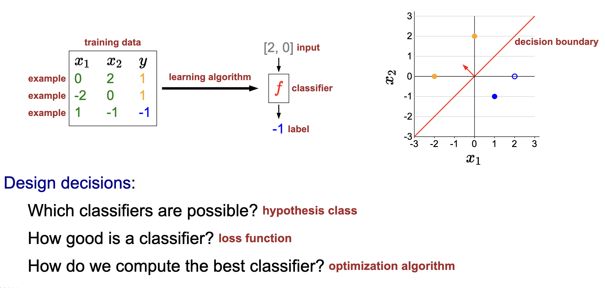
- Binary linear classifier: \(f_{\mathbf{w}}(x)=\operatorname{sign}(\mathbf{w} \cdot \phi(x))\).
- Hypothesis class: \(\mathcal{F}=\left\{f_{\mathbf{w}}: \mathbf{w} \in \mathbb{R}^2\right\}\).
- Loss:
- zero-one: \(\operatorname{Loss}_{0-1}(x, y, \mathbf{w})=\mathbf{1}\left[f_{\mathbf{w}}(x) \neq y\right]\)
- If correct classification, loss is 1. Else, loss is 0.
- hinge: fixing the problems with the zero-one loss.
- zero-one: \(\operatorname{Loss}_{0-1}(x, y, \mathbf{w})=\mathbf{1}\left[f_{\mathbf{w}}(x) \neq y\right]\)
Score and margin
Detour. New concepts.
Definition 5 Score:
- In regression, this is just the prediction (model output).
- In classification, confidence in which we are predicting (+1):
- The score on an example \((x, y)\) is \(\mathbf{w} \cdot \phi(x)\), how confident we are in predicting \(+1\).
- This essentially is the number before taking the sign in the prediction from the model.
- The score on an example \((x, y)\) is \(\mathbf{w} \cdot \phi(x)\), how confident we are in predicting \(+1\).
Definition 6 (Margin):
- The margin on an example \((x, y)\) is \((\mathbf{w} \cdot \phi(x)) y\), how correct we are. Score times \(y\).
- More: larger the margin, the more correct. If \(y=1\), then score (raw prediction) needs to be very high to have good margin. Vise versa if \(y=-1\).
Note that these concepts help us delve deeper into the nuances of the classifer as opposed to just seeing whether the predictor is right or wrong. This will help us transform the zero-one loss into hinge.
Problems with zero-one loss:
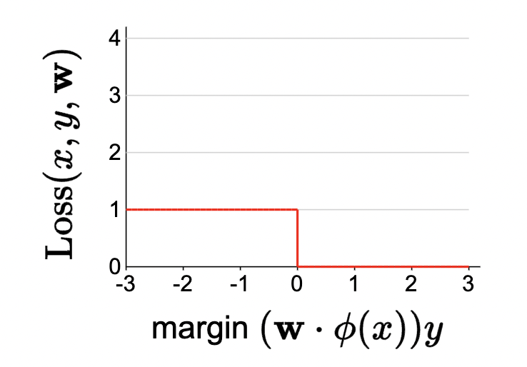
- non-differentiable
- flat curve means zero-gradients almost everywhere: thus, GD will get stuck!
Introducing hinge loss
To resolve the above problems, we now introduce the hinge loss.
Definition 7 (Hinge loss)
- In words: the maximum over a descending line and the zero function. In other words,
- If the margin is at least 1, then the hinge loss is zero.
- If the margin is less than 1, then the hinge loss rises linearly.
- In math:
\[\operatorname{Loss}_{\text {hinge }}(x, y, \mathbf{w})=\max \{1-(\mathbf{w} \cdot \phi(x)) y, 0\}\]
- Now visually:
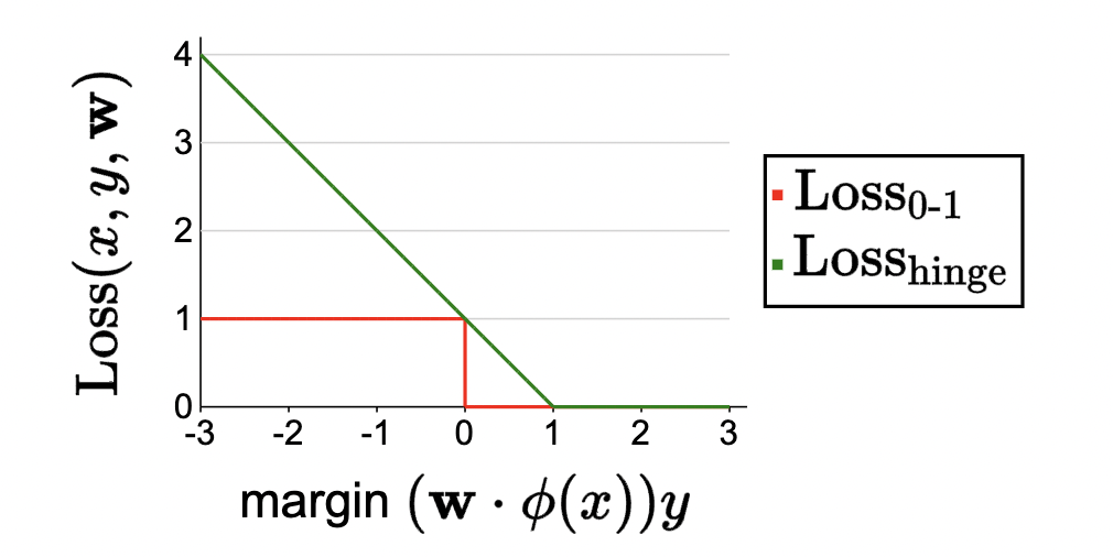
Some intuitions:
- Hinge loss is upper bound of zero-one (see this visually). So if we drive down hinge loss, we must also be driving down zero-one.
- Logistic is another common loss to use here.
Module: Stochastic Gradient Descent (Offline)
Problem with gradient descent (it is too computationally expensive and slow!):
- In regular gradient descent (see Definition 4), we update the weights after every epoch by summing all of the losses for each datum in the dataset. This is expensive since, for each iteration, just to update the weights, we must traverse the entire dataset. And for large problems, we should we updating the weights quite often.
- Also, “recall that the training loss is a sum over the training data. If we have one million training examples, then each gradient computation requires going through those one million examples, and this must happen before we can make any progress” (CS 221 Slides).
Thus, we introduce:
Definition 8 (Stochastic Gradient descent):
- Initialize \(\mathbf{w}=[0, \ldots, 0]\)
- For \(t=1, \ldots, T\) : epochs
- For \((x, y) \in \mathcal{D}_{\text {train }}\):
- \(\mathbf{w} \leftarrow \mathbf{w}-\eta \nabla_{\mathbf{w}} \operatorname{Loss}(x, y, \mathbf{w})\)
- For \((x, y) \in \mathcal{D}_{\text {train }}\):
Differences and notes:
- We aren’t differentiating \(\operatorname{TrainLoss}(\mathbf{w})=\frac{1}{\left|\mathcal{D}_{\text {train }}\right|} \sum_{(x, y) \in \mathcal{D}_{\text {train }}} \operatorname{Loss}(x, y, \mathbf{w})\). Just \(\operatorname{Loss}(x, y, \mathbf{w})\).
- We update the weights on a per-sample, rather than per-epoch basis.
- Drawback: each update isn’t as good/general since we are only looking at one sample when updating. But more efficient this way.
- Thus, can become unstable. Here is happy medium:
- Mini-batch SGD: per-batch basis instead of per-sample. i.e., take gradient averages over \(B\) samples per weight update.
- Can add randomization regularization: randomize the order of the dataset for each epoch.
(Stochastic gradient descent in python):
def stochasticGradientDescent(f, gradientf, n, initialWeightVector):
    w = initialWeightVector()
    numUpdates = 0
    for t in range(500):
        for i in range(n):
            value = f(w, i)
            gradient = gradientf(w, i)
            numUpdates += 1
            eta = 1.0 / math.sqrt(numUpdates)
            w = w - eta * gradient
        print(f'epoch {t}: w = {w}, F(w) = {value}, gradientF = {gradient}')
Credit: CS 221.
Step size
\[\mathbf{w} \leftarrow \mathbf{w}-\underbrace{\eta}_{\text {step size }} \nabla_{\mathbf{w}} \operatorname{Loss}(x, y, \mathbf{w})\]
aka learning rate.
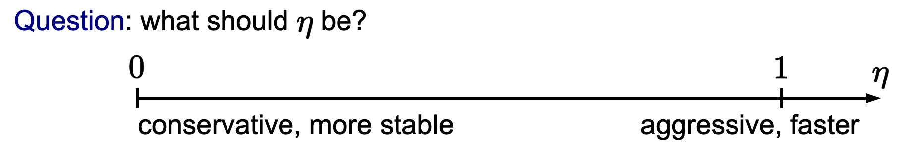
- How do we choose this in practice?
- Analogy: step sizes are like driving: larger step size might mean getting there faster but can also crash and burn.
- On the other hand, smaller SS will increase stability but get us there much slower. Note that if \(\eta = 0\), then \(\mathbf{w}\) is actually never updated.
- Adaptive strategy:
- set the initial step size to \(\mathbf{1}\) and let the step size decrease as the inverse of the square root of the number of updates we’ve taken so far.
- Asides:
- Adam and Adagrad are more advanced and tweak this based on your data.
- Theoretical results prove SGD convergence given that gradients are bounded with your data.
Footnotes
Question: when we say “learning” algorithm, what are we referring to? The whole framework? Backprop?↩︎
is this always the case though?↩︎
Question: I am still confused on the difference between score and margin. Is margin measures correctness, what is the difference between margin and loss then?↩︎
see how plotting the loss against the margin allows us to discover the following pitfalls? (motivation for introducing margin).↩︎