Reference
6-10. Random variables
Approximations
- Use the Poisson approximation when \(n\) is large \((>20)\) and \(p\) is small \((<0.05)\). Use the Normal approximation when \(n\) is large \((>20)\), and \(p\) is mid-ranged. Specifically, when variance is greater then 10 , in other words: \(n p(1-p)>10\). If in doubt, go with normal.
12-13. Bayes’ and conditional probability with random variables
Discrete/discrete conditional: \(X\) and \(Y\) are discrete RV’s. Conditional definition with discrete random variables. \[ \mathrm{P}(X=x \mid Y=y)=\frac{P(X=x, Y=y)}{P(Y=y)} \]
Discrete/discrete Bayes’: Let \(M\) and \(N\) be discrete random variables. Then, by Bayes’ theorem: \[P(M=m \mid N=n)=\frac{P(N=n \mid M=m) P(M=m)}{P(N=n)}.\] Law of total probability way: \[P(M=m \mid N=n)=\frac{P(N=n \mid M=m) P(M=m)}{P(N=n \mid M=m) P(M=m) + P(N=n \mid M=m^{C}) P(M=m^{C})}.\]
Bayes’ formulas
\[ \mathrm{M}, \mathrm{N} \text { are discrete. } \mathrm{X}, \mathrm{Y} \text { are continuous } \]
\[ \begin{aligned} p_{M \mid N}(m \mid n) &=\frac{P_{N \mid M}(n \mid m) p_{M}(m)}{p_{N}(n)} \\ f_{X \mid N}(x \mid n) &=\frac{P_{N \mid X}(n \mid x) f_{X}(x)}{P_{N}(n)} \\ p_{N \mid X}(n \mid x) &=\frac{f_{X \mid N}(x \mid n) p_{N}(n)}{f_{X}(x)} \\ f_{X \mid Y}(x \mid y) &=\frac{f_{Y \mid X}(y \mid x) f_{X}(x)}{f_{Y}(y)} \end{aligned} \]
14-15. General inference (Bayesian networks)
- We started out with joints for specifying various probabilities for multiple random variable systems. However, joint becomes too big so we to do inference (conditional probability RVs: updating your belief about an RV event given a different RV event), we construct causal Bayesian networks. To compute conditional probability from Bayesian network, use rejection sampling: Pseudcode:
- Step 0: Have a fully specified Bayesian network layed out.
- Step 1: sample a ton!
- Step 2: collect subset of samples consistent with observation (thing you are conditioning)
- Step 3: loop through this subset and count number of times the thing you want the probability of is present in the sample.
- Step 4: Divide this count by the length of this sample subset (the subset whose elements are samples consistent with the observation).
16. Beta
Uniform prior:

Conjugate prior:

19. Bootstrapping
Summary: say we want to measure a statistic about the general population. We of course cannot survey the entire population so instead we take a sample of size \(n\). Then, bootstrapping allows us to estimate what the true distribution (i.e. if the whole population had indeed been sampled) is by resampling. Specifically, the algorithm goes like this: 1. take your initial sample from the population of size \(n\). 2. Create a loop of 10,000 or greater times. At each iteration, draw a sample, of size \(n\) from the initial sample. 3. Calculate your statistic you want on this subset sample. Append it to a master list. 4. After the loop, calculate the statistic on this master list itself (note that the master list is literally a graph-able list of all the e.g. variances and from that distribution you want the e.g. variance). This is you answer.
Pseudocode:
def bootstrap(sample):
   N = number of elements in sample
   pmf = estimate the underlying pmf from the sample
   stats = []
   repeat 10,000 times:
      resample = draw N new samples from the pmf
      stat = calculate your stat on the resample
      stats.append(stat)
   stats can now be used to estimate the distribution of the stat
P-values
We have two distributions of numbers. We want to know whether or not the two distributions are fundamentally different or the same: were the numbers for each distribution drawn from the same universal underlying distribution? - The null hypothesis is that they aren’t different: there is no difference between the two groups, so everyone is drawn from the same distribution. A p-value is simply the probability (i.e. # between \([0,1]\)) that the null hypothesis is true. So…
- If \(p\) is closer to \(1\), then we think that the distributions are likely to be the same (i.e. drawn from the same underlying distribution).
- If \(p\) is closer to \(0\), then we think that the distributions are likely to be different (i.e. drawn from different underlying distributions).
We use bootstrapping here via repeated sampling.
First, take the two distributions and jot down the initial difference between the means (or whatever relevant statistic you are calculating). 1. Concatenate together the two sample lists to make one universal distribution, \(U\). 2. Iterate at least \(10,000\) times and at each iteration, sample from \(U\) (appropriate lengths) twice: one for group A and one for group B. 3. Say you want to calculate the difference in means (called effect size). Take abs(diff between means). Append this to a master list which gets all the effect sizes for the iterations. 4. Also, at each iteration, calculate whether the effect size between the current sample means is greater than the initial effect size. If so, add to a counter. 5. At the end, take the counter value and divide it by the total number of iterations. This is your p-value.
We can calculate p-value using bootstrapping:
- Identify what sample statistics you’re calculating, e.g. abs difference of sample means.
- State null hypothesis.
- Calculate observed sample statistics (using observed sample).
- Run a bootstrap experiment.
- Resample the original sample to get a equally-sized new sample.
- Calculate new sample statistic.
- If new sample statistic is more extreme than observed statistic, count \(+=1\).
- p-value: percentage of more extreme samples over all bootstrap samples \(\left(\frac{\text { count }}{\text { num trials }}\right)\).
Alternative explanation:
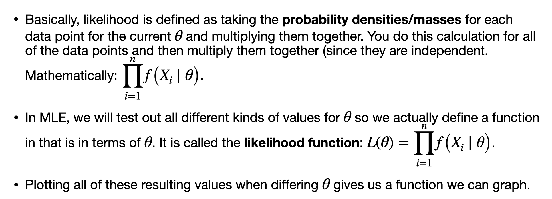
Maximum likelihood estimation (MLE)
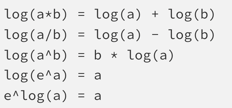
Logarithm rules
Recall we are working with \(log_e\) (natural log) which is \(ln\). 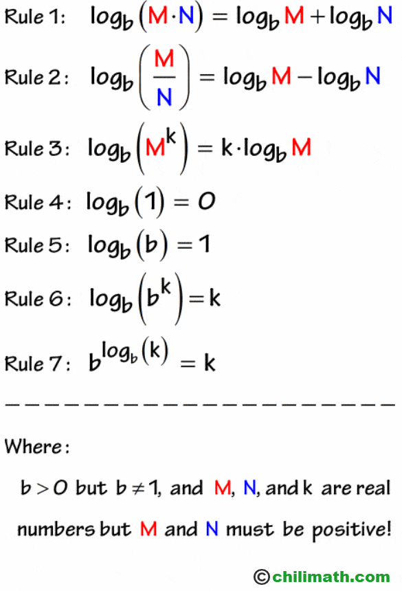
Derivative rules:
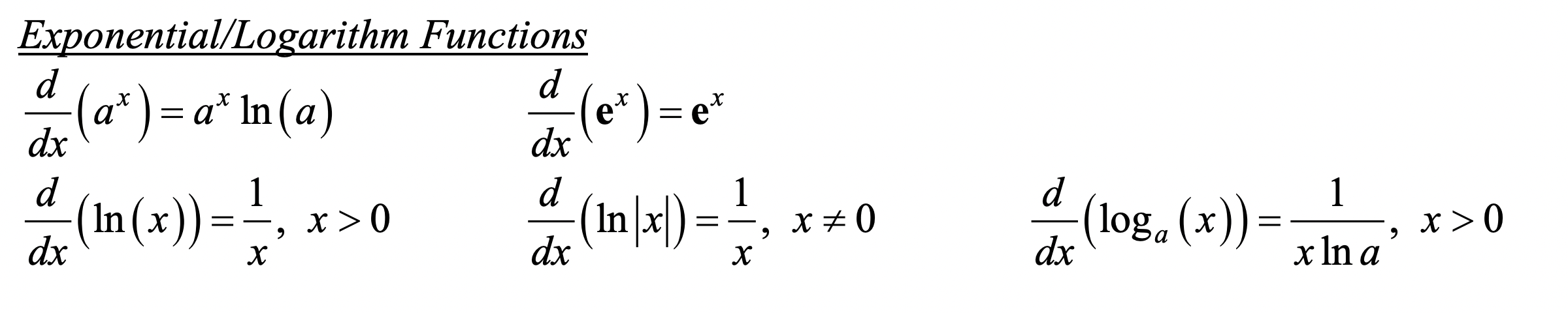
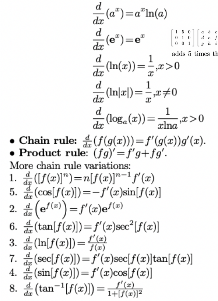
\[ \begin{aligned} &\frac{d}{d x} \ln (x)=\frac{1}{x} \\ &\frac{d}{d x} \ln [f(x)]=\frac{1}{f(x)} f^{\prime}(x) \\ &\frac{d}{d x} \log _{a}(x)=\frac{1}{x \ln a} \\ &\frac{d}{d x} \log _{a}[f(x)]=\frac{1}{f(x) \ln a} f^{\prime}(x) \end{aligned} \]
17. Adding random variables
- Example: here is an intuitive example. We have two groups of people
- P1: 50 people, each independently infected with \(p=0.1\)
- P2: 100 people, each independently infected with \(p=0.4\)
- Question: Probability of more than 40 infections?
- Solution: your first thought is probably to define two binomial random variables and just add them. Let \(P_1 \sim bin(50,0.1)\) and let \(P_1 \sim bin(100,0.4)\). But we have a problem. We can’t add binomials with different probability parameters (see course reader equation definitions)! So what we do now? We approximate the binomials with normals!!!
- The key point here is that you should try to rearrange your problem to get it in terms of something you know how to work with.
- Though remember to perform continuinty correction when tranforming from the discrete to continious realm.
- Solution: your first thought is probably to define two binomial random variables and just add them. Let \(P_1 \sim bin(50,0.1)\) and let \(P_1 \sim bin(100,0.4)\). But we have a problem. We can’t add binomials with different probability parameters (see course reader equation definitions)! So what we do now? We approximate the binomials with normals!!!
- Remark: Say we have some random variable, \(X\). What is \(2X\)? Hold your horses. It is not like what we did above. In fact, this is an invalid expression. Can you picture why? Because \(X\) is not independent from itself! So instead, we must use a linear transform.
- Remark: subtraction is just addition by linear transforming the second part of the expression with -1 first. So \(X-Y=X+(-1Y)=X+(-Y)\).