Lecture 24: Logistic Regression
We now look at another powerful classification algorithm called logistic regression.
- “Heart and soul” of neural networks
- Optimization:
- We need to understand optimization because Log reg., uses it quite heavily!
The idea behind supervised learning is, training data in form \((\mathbf{x}, y) \ldots\) we want to learn function \(\hat{y}=g(\mathbf{x})\) that maps \(\mathbf{x}\) to \(y\). This is the same thing as \(g(\mathbf{x})=\operatorname{argmax} \hat{P}(Y=y \mid \mathbf{X})\). IN Naive Bayes’ we literally worked directly with this probability and manipulated it using Bayes’. Here we take a different approach. We recognize that this is just one big function that maps \(\mathbf{X} \rightarrow y\). We are going to try to “approximate” this function!
0. Background and notation
Before we get started, we need to introduce a couple new things and notation: 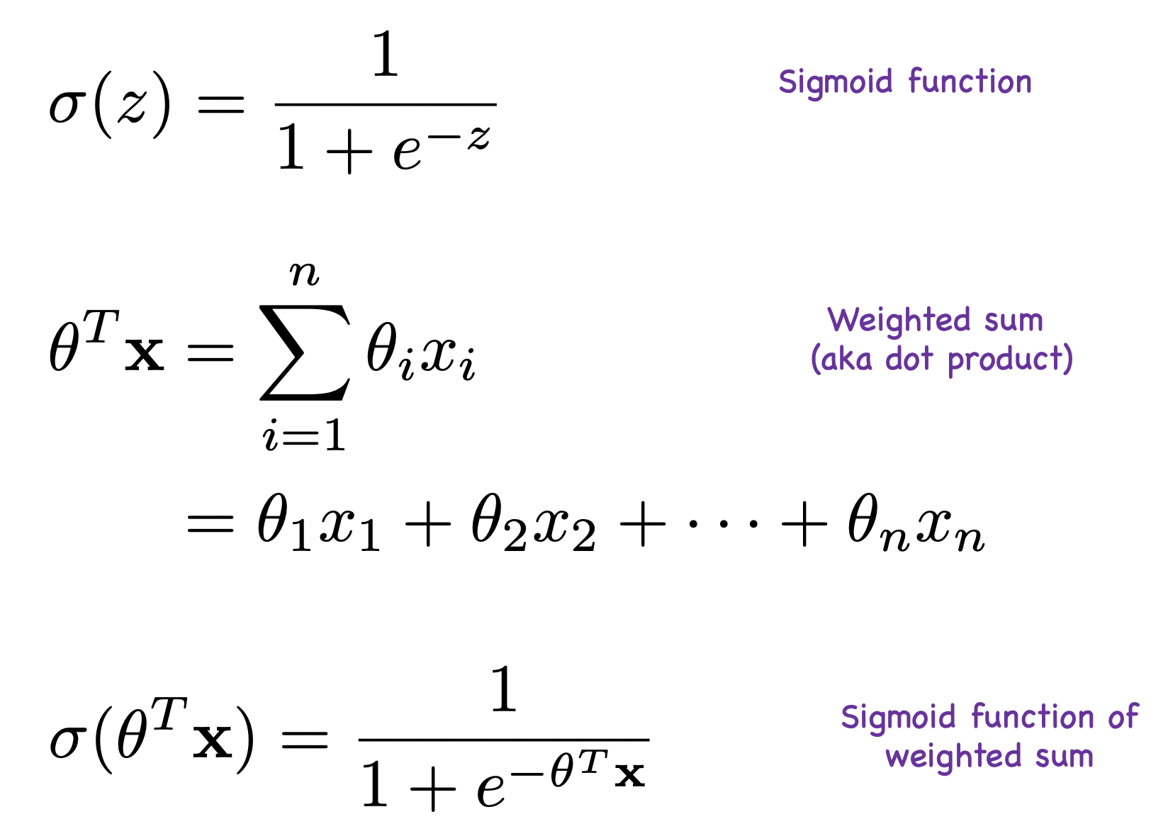
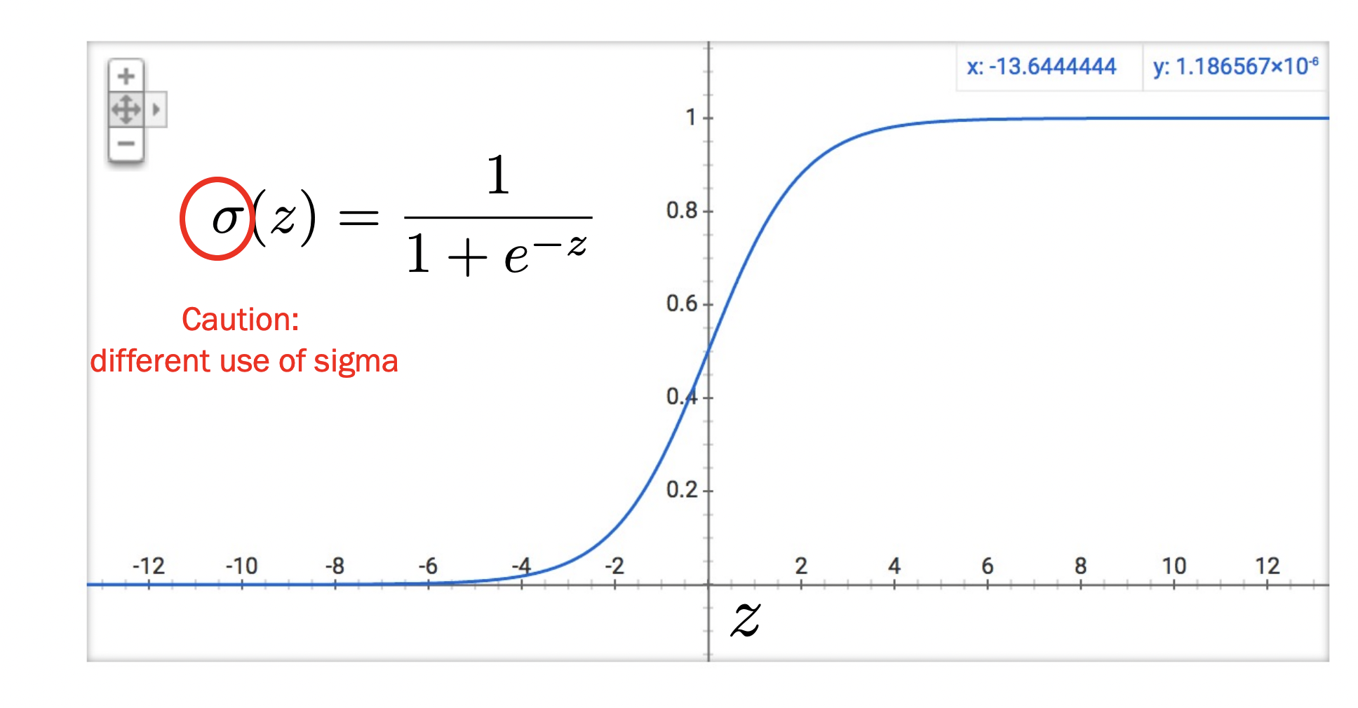
- The sigmoid function is a squashing function which squashes input \(z\) to be a number between 0 and 1 (needed for probabilities!). It looks like:
- Second, we will be doing lots of matrix-vector multiplications here because of weighted sums. So it is important to understand the inner/dot product between parameters and inputs: \[\begin{array}{rlr} \theta^{T} \mathbf{x} & =\sum_{i=1}^{n} \theta_{i} x_{i} \quad \begin{array}{c} \text { Weighted sum } \\ \text { (aka dot product) } \end{array} \\ & =\theta_{1} x_{1}+\theta_{2} x_{2}+\cdots+\theta_{n} x_{n} \end{array}\]
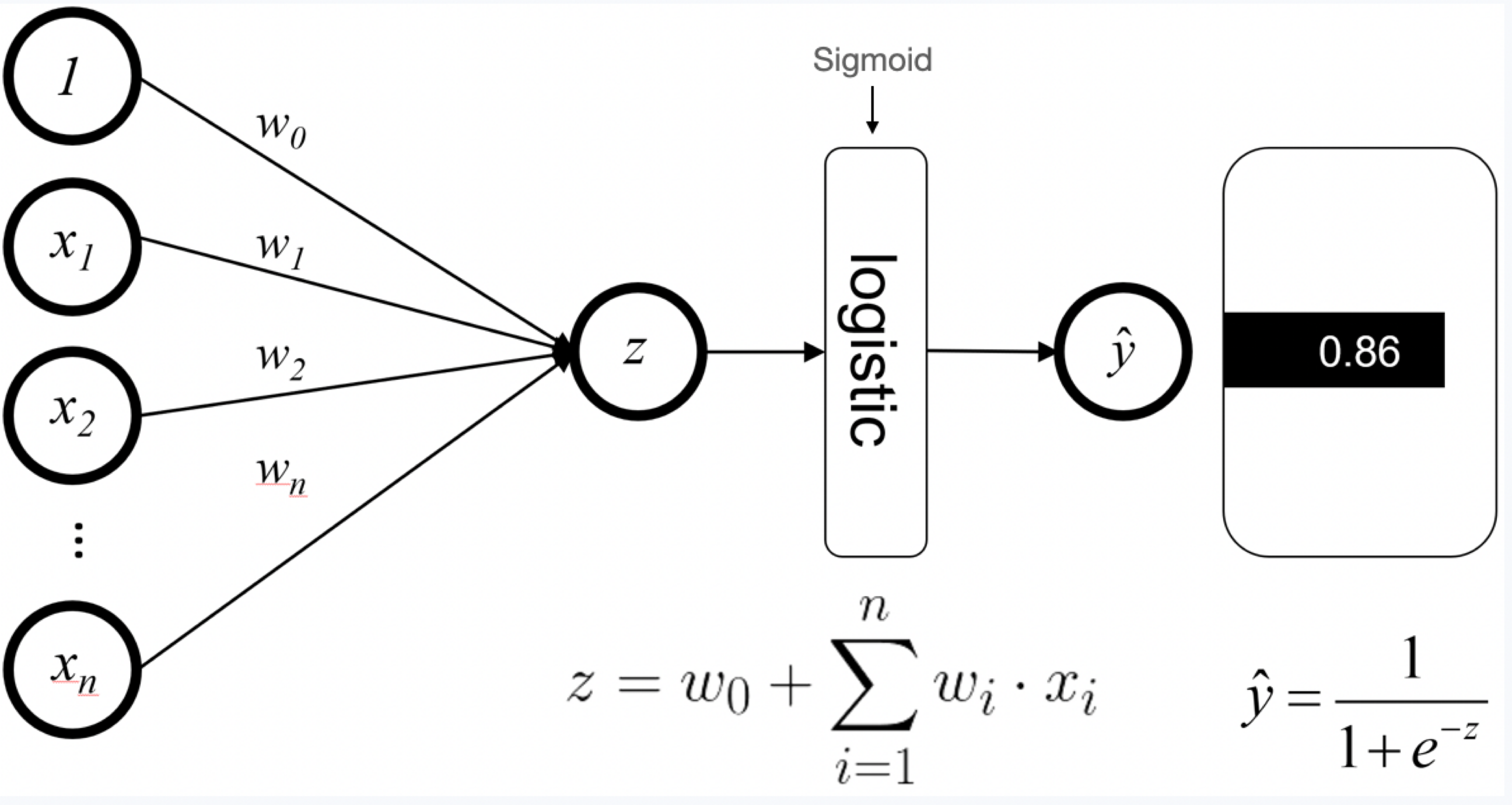
- And finally, we put these two together in the third point. The reason is what we will be doing is (2.) computing the weighted sum and then (1.) squashing it to a probability. Directly, we define this as \(\sigma\left(\theta^{T} \mathbf{x}\right)=\frac{1}{1+e^{-\theta^{T} \mathbf{x}}}\).
Also, some calculus background:
- Recall that for composition of functions, \(f(x)=f(z(x))\), we use chain rule: \[ \frac{\partial f(x)}{\partial x}=\frac{\partial f(z)}{\partial z} \cdot \frac{\partial z}{\partial x}. \]
1. Big picture
- NB made a naive assumption. That leaves room for improvement!
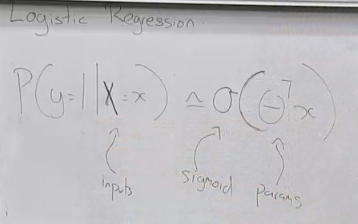
- Cut to the chase! Avoid probabilities. Just approximate the function \(P(Y \mid X)\)! In other words: \[P(Y=1 \mid \mathbf{X}=\mathbf{x})=\sigma\left(\sum_{i} \theta_{i} x_{i}\right)\].
- You can think of this as a rule-based machine guided by some weighted: you stick in an input, it gets weighted by the parameters (sliders), summed up and squashed.
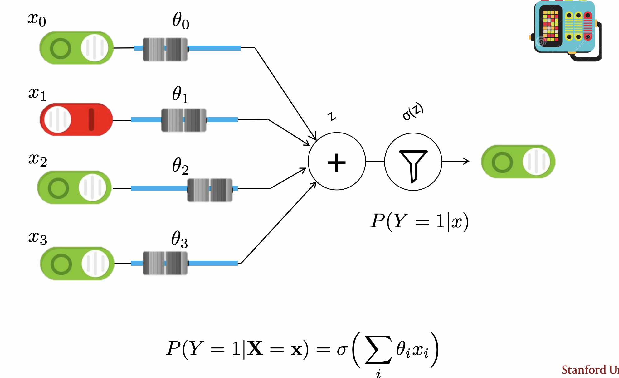
- In other words, we are just using a direct engineering approach: no probability theory (yet)! In actuality, this is just a neural network with no hidden layers!
- But of course, our outputs depend on those weights. So we are going to use prob. and calculus to estimate them!
- Small note: we add an extra input that is always “turned on (i.e. in binary, the feature is always a 1)” to make it work a little better. This is called a “bias” term.
Math: this equation is how we “predict” on a new test sample \(\mathbf{x}\): \[P(Y=1 \mid \mathbf{X}=\mathbf{x})=\sigma\left(\sum_{i} \theta_{i} x_{i}\right).\]
that is literally it! Nothing else to it. Except of course, we need to determine what exactly these \(\theta_i\)’s (parameters/weights) are. We have a method for this: parameter estimation! MLE!
So once we have these \(\theta_i\)’s determined from training, we basically have this rule-based machine that we can use to make predictions with ease!
Of course though, the hard part is determined these \(\theta_i\)’s. We do this via training which is what we get into next.
- Key note: \(P(Y=1 \mid \mathbf{X}=\mathbf{x})=\sigma\left(\sum_{i} \theta_{i} x_{i}\right)\), is, as stated, a probability for \(y=1\) so to get \(P(Y=0 \mid \mathbf{X})\) we just employ the law of total probability and subtract from this.
We have discussed the forward pass now lets do the backwards pass!
- Note: a cool thing about Sigmoid is that it basically turns the “energy” (weighted sum) coming into the probability into a thing that functions like a probability.
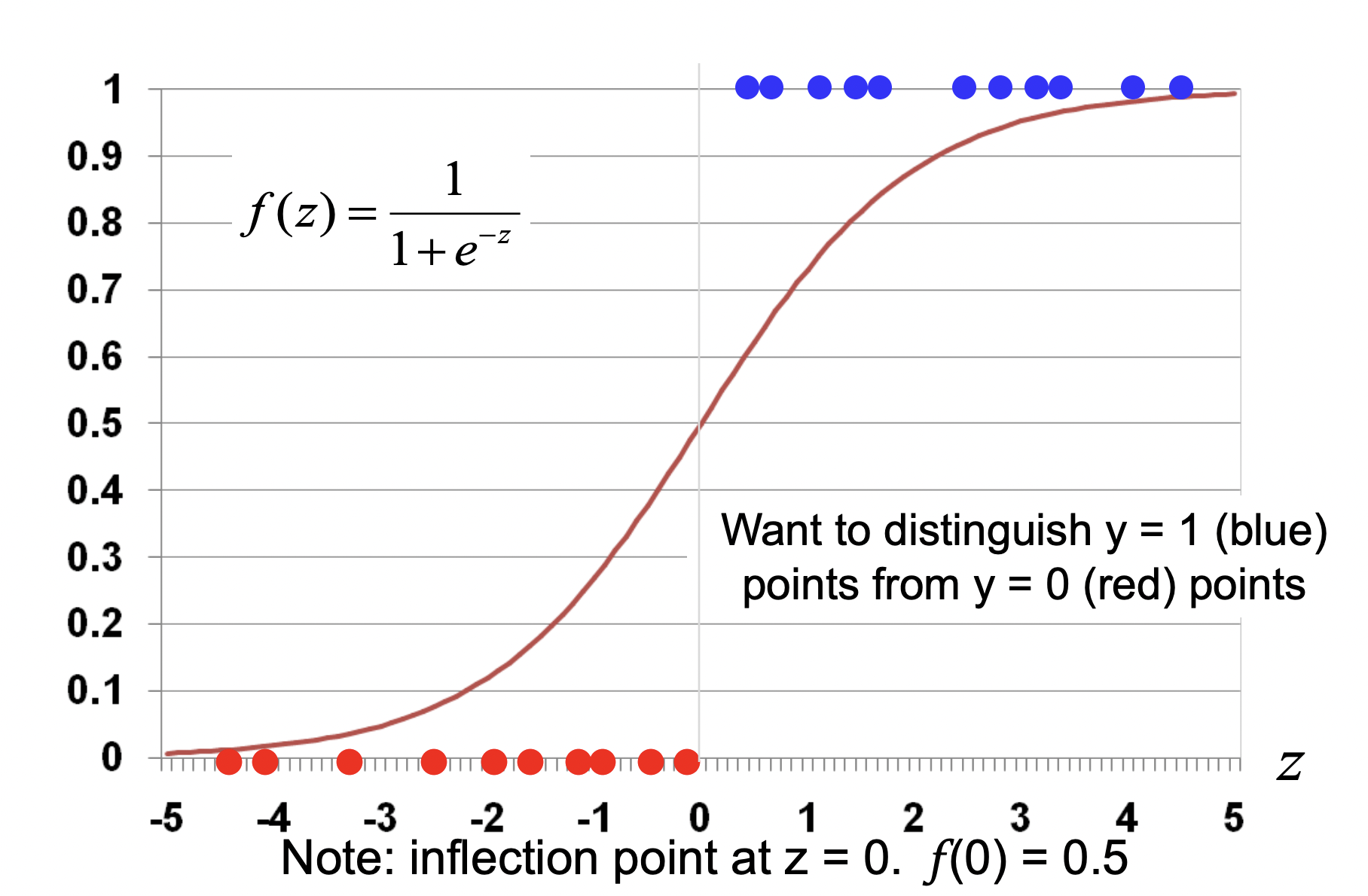 See how the inflection point is at \(y=0.5\)? So any positive energy will be predicted positively and vise versa.
2. Training the weights
- Our performance in predicting new samples will be based on the values of the weight parameters. So that is where the real intelligence comes from: estimating the weight values! How do we do this? Let’s find out!
- We are going to use MLE: we need to find the parameters that make our data look most likely!
- But of course, we don’t have a direct distribution we are using as a model. So what are the parameters we are estimating? Well, we don’t need a defined distribution. We just want to estimate those weights–those are the these parameters.
- Recall that MLE is taking derivatives.
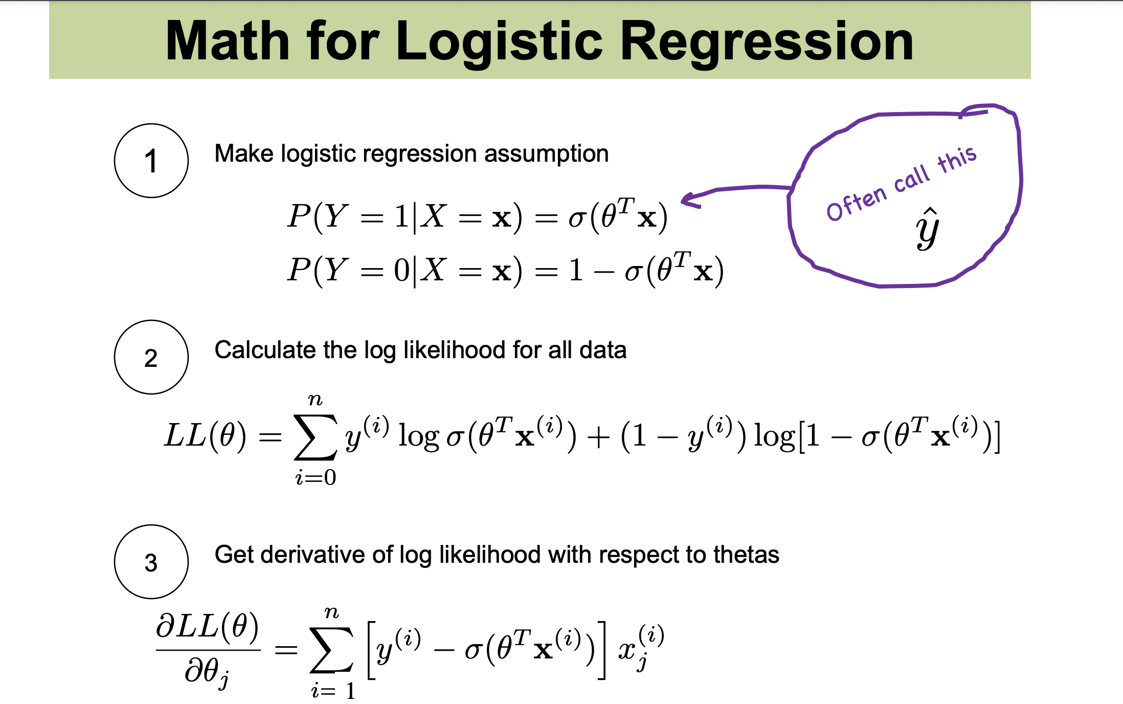
We use gradient ascent and update our gradient using the last line in this formula. We have multiple weights so we actually calculate the gradient for all of these weights and update them for each one on each iteration. Thus, we have a for loop for each iteration (double for-loop).
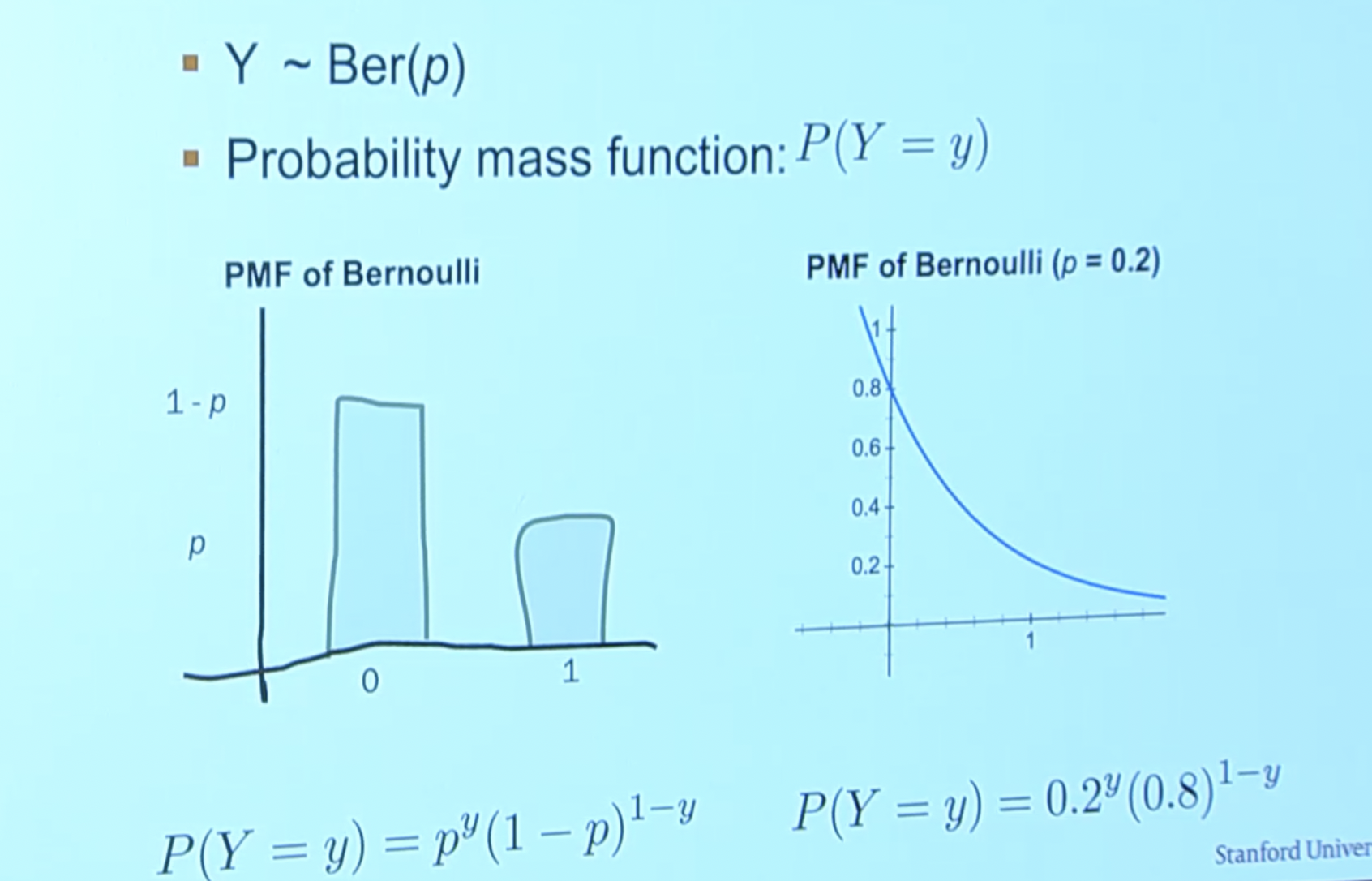
- Cool (i.e. how we derived the LL function above): in binary classification, we essentially just have a Bernoulli! But that isn’t differentiable so we model it in a continious fashion:
 .
.
So we just plug in \(P(Y=1 \mid \mathbf{X}=\mathbf{x})=\sigma\left(\sum_{i} \theta_{i} x_{i}\right)\) for \(p\) in the Bernoulli continious equation.