🛶 Lecture 22: Maximum A Posteriori
- Our goal in ML is to estimate the parameters of a distribution.
- We learned of a nice technique called MLE last lecture. But it can get quite limited in certain scenarios. So we introduce another one here called (Maximum A Posteriori) to add to our repertoire.
Problems with MLE
- Take a uniform distribution… it will just learn the min and max vals as the parameters. But that is nonsense: every point’s probabilities aren’t uniform! The problem? MLE overfits. It doesn’t generalize well to new data.
Intro to MAP
- The philosophy is that we do want to incorporate prior information that we know about the world into our estimations.
Difference (see 1:02): - MLE: choose the parameters (\(\theta\)) that makes your data look most likely: \(L(\theta)=\prod_{i=1}^{n} f\left(X_{i} \mid \theta\right).\) \[\begin{aligned} \hat{\theta}_{M L E} &=\underset{\theta}{\operatorname{argmax}} f\left(X^{(1)}=x^{(1)}, \ldots, X^{(n)}=x^{(n)} \mid \theta\right) \\ &=\underset{\theta}{\operatorname{argmax}}\left(\sum_{i} \log f\left(X^{(i)}=x^{(i)} \mid \theta\right)\right) \end{aligned}.\] - MAP: choose the most likely parameters, \(\theta\), given the data \(X_{1}, X_{2}, \ldots, X_{n}\). \[\hat{\theta}_{M A P}=\underset{\theta}{\operatorname{argmax}} f\left(\theta \mid x^{(1)}, \ldots, x^{(n)}\right).\]
Deriving the MAP
So… we know how to do \(\underset{\theta}{\operatorname{argmax}} f(X \mid \theta)\) (MLE) but now we want the opposite: \(\underset{\theta}{\operatorname{argmax}} f(\theta \mid X)\). This should scream Bayes! Because it doesn’t make much sense to calculate the most likely parameters, \(\theta\), given the data. But the inverse is easy so we use Bayes’:
\[\hat{\theta}_{M A P}=\underset{\theta}{\operatorname{argmax}} \frac{f\left(x^{(1)}, x^{(2)}, \ldots, x^{(n)} \mid \theta\right) g(\theta)}{h\left(x^{(1)}, x^{(2)}, \ldots x^{(n)}\right)}. \]
Notice that we have the MLE part as our likelihood (quite a fitting name!) and also that a whole new prior is included. How do we get that? That is for you to choose and incorporate into your model! You see how this is more powerful now? We can input another prior! We are going to choose a \(\theta\) that is informed by our prior belief.
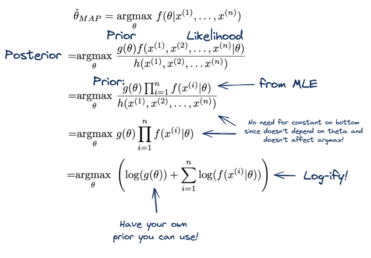
Ah… look how nice that is… we literally end up with the same equation except now we can incorporate our prior beliefs as well! Yippee! It’s quite conveniant.
- Note: the prior is a “prior belief in the parameter \(\theta\)”. So this is a probability of the parameter (not just the parameter itself). So let us say you have a Bernoulli you want to estimate the parameter \(p\) for. Your prior should be your prior belief in \(p\) which itself is a probability. So we have a probability of a probability. And therefore, we choose to represent our prior using the Beta distribution.
- Definition (Laplace prior): When using a beta as a prior, we can use our expert domain knowledge to determine the parameters of that beta prior. But sometimes we don’t have expert domain knowledge so a common one to start out with as a base is to say you observed 1 success, 1 failure: so the prior is \(beta(2,2)\). Doing this prevents any posterior probability from being 0 or 1 (useful for programming so you don’t fuck up computation!). Recall Hamilton Federalist paper example: if there was one singular word in the document that Hamilton never wrote before…. BAM! probability for Hamilton writing that document drops all the way to 0! So use Laplace prior for cases like this (like in your project!).
- Note: we do NOT train the prior’s parameters. These are chosen by us (that is the whole point on “updating your prior beliefs”… these are beliefs you already hold).
- Definition (Laplace prior): When using a beta as a prior, we can use our expert domain knowledge to determine the parameters of that beta prior. But sometimes we don’t have expert domain knowledge so a common one to start out with as a base is to say you observed 1 success, 1 failure: so the prior is \(beta(2,2)\). Doing this prevents any posterior probability from being 0 or 1 (useful for programming so you don’t fuck up computation!). Recall Hamilton Federalist paper example: if there was one singular word in the document that Hamilton never wrote before…. BAM! probability for Hamilton writing that document drops all the way to 0! So use Laplace prior for cases like this (like in your project!).
Note: see
23:00-27:00and make notes on that part where he talks about which priors to use for what posteriors (i.e we are actually estimating the posterior’s parameters).