🌋 Lecture 21: Maximum Likelihood Estimation
https://www.cs.cmu.edu/~tom/mlbook/
We now turn to machine learning and we begin with MLE where we try to estimate the parameters for a parametric distribution based on some observed data. But to understand this, we first need a thorough understanding of what exactly is likelihood and some other probabiltiy basics.
Review: what is likelihood?
- We aim to understand the differences between probability and likelihood. We begin with reviewing how we came about random variables and probability. Say that there exists some random process such as coin flipping (e.g. outcomes of tossing a coin 10 times). In such cases, to gain a deeper intuition for the process, we assign a random variable to the process and calculate probabilities for how probable it is that the RV takes on a certain value. In such cases, we can calculate the probability of observing a particular set of outcomes by making suitable assumptions about the underlying stochastic process. For example, we might be given that the coin comes up heads with probability \(\theta = p = 0.4\) per one flip. Thus, we can calculate \(P(X=x \mid \theta)\) where \(\theta\) is that probability parameter. Now you might be wondering, where do we get \(\theta\) from? Do we just pull it out of our ass (excuse the French)? See, in the real world, we often do not know what the \(\theta\) is and it isn’t just given to us. Instead, what we do have is the ability to flip the coin some \(n\) times and from that, we can calculate the \(\theta\). That is, we simply observe the process that \(X\) is representing and the goal then is to arrive at an estimate for \(\theta\) that would be a plausible choice given the observed outcomes from \(X\). To do this in a structured way, we represent this as a function of \(\theta\) and it is defined as \(L(\theta \mid X)\): the notation makes sense, we want to know \(\theta\) given the outcomes we observe from \(X\). Such a function is called the likelihood.
- Let us probe this further: \(L(\theta \mid X)\) means “how likely are we to see a certain distribution given the obersevations?”. For example, in the normal case,
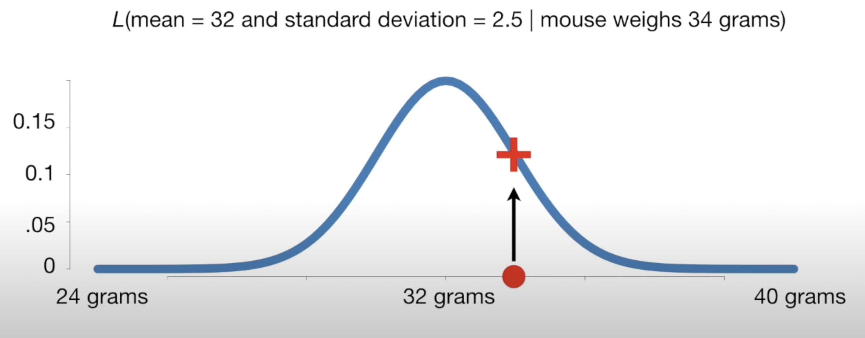
- Here we ask, how likely is it that the normal distriubtion follows this exact curve given the observed data (that the mouse weighs 34 grams)? So in some ways, we are composing the distribution curve based on the data! How do we compose such a curve? We first make an assumption for the parametric form it fits. Then, we estimate the parameters. This forms the curve. So likelihood, defined as \(L(\theta \mid X)\), is simply how likely is it that the curve is shaped like this given the observed data. That is the semantic meaning and it is quite different than probability (i.e. doesn’t have to be between 0 and 1). In this lecture, we show how to estimate such parameters so that the curve is most likely given the data. The reasoning for this is that the experiment is a full circle: we can then use the constructed distriubution to make future predictions on probabilities!
- Here is a nice math result: \(L(\theta \mid X)=P(X \mid \theta)\): it turns out that the likelihood of a distribution given the data is the same as the probability density of the outcome given the distribution (see here). First answer here is also good and of course StatQuest. Notice in the StatQuest video that he explains likelihood by shifting around the normal curve until the likelihood is maxed out (i.e. it fits the data observed well).
- A note: it is vital to understand the realtion \(L(\theta \mid X)=P(X \mid \theta)\). Specifically, \(P(X \mid \theta)\) means the probability that we would observe our data \(X\) given the parametric distribution \(\theta\). This is the same thing as saying how likely is it that our distribution is constructed with parameters \(\theta\) given the data we observed. See why?
- Let us probe this further: \(L(\theta \mid X)\) means “how likely are we to see a certain distribution given the obersevations?”. For example, in the normal case,
- Notice how this is a full circle: we have some underlying random process to which we want a whole distribution of probabilities for what the process outcome may be. However, we have no intuition yet so to derive the parameters for the distribution, we need to observe some data in real life. From this, we get the parameters we need to form our probabilistic intuitions.
In my own words,
Likelihood: the likelihood is defined as how likely is it that the given parametric distribution curve (i.e. the parameters for the assumed parametric distribution family) is the correct probability distribution for the the data that has been observed.
MLE: so MLE is the process of calculating the best curve for the distribution to fit the data: that is, maximizing \(L(\theta \mid X)\).
Another mental model for likelihood: say we have some data and a dsitribution curve. Now let us draw a few samples from the distribution. Likelihood measures how likely it is that the observed data matches the drawn samples. i.e. how probable is it that we’d draw samples matching the observed data? This should help you understand \(L(\theta \mid X)=f(X \mid \theta)\).
 The probability that we’d observe
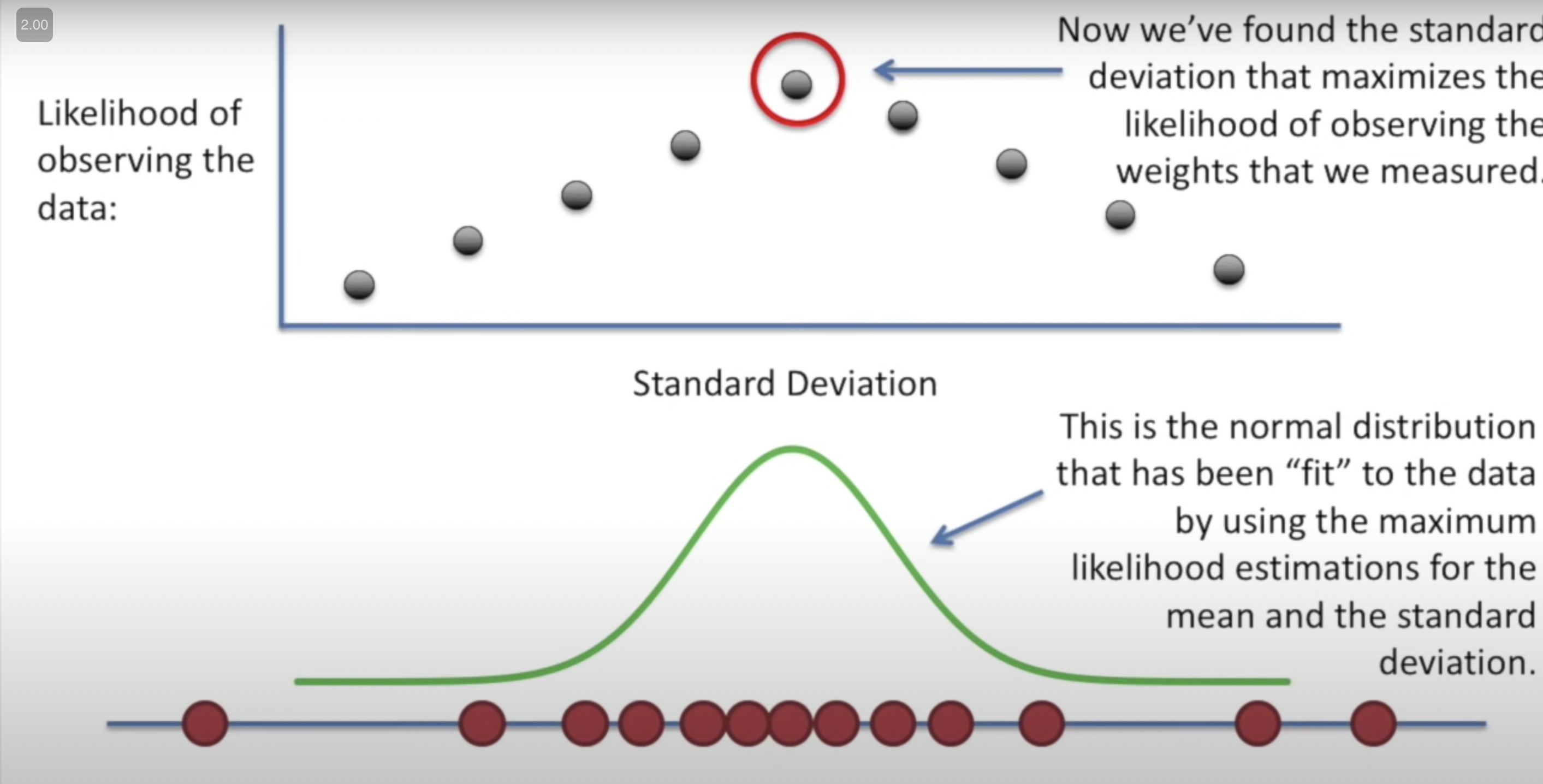
I mean this makes sense: what is the probability of observing your data given the parameters for the distribution (this is how likelihood is defined in course textbook: \(L(\theta)=\prod_{i=1}^{n} f\left(X_{i} \mid \theta\right)\). We want this probability to be as high as possible so that the resultant curve is fit well to the actual data. If we take a bunch of different values for \(\theta\) (x-axis) and plot the results (y-axis) of the above equation on a graph, we get the likelihood function. We aim to find the maximum value of this function.
Ok… actual lecture notes now.
- Basically, likelihood is defined as taking the probability densities for each data point for a certain \(\theta\) and multiplying them together. Now do this for a bunch of different \(\theta\) values. This is the likelihood function. See
49:00from lecture.- From this, it is easy to see that \[L(\theta)=\prod_{i=1}^{n} f\left(X_{i} \mid \theta\right).\]
- We don’t lile products and it gets small so we just use log of likelihood.
Ok so we need to maximize LL function. How to do? Gradient ascent!
Discrete to continious
A note: discrete to continious. We have things in terms of densities so we will work with discrete for everything. The good news is that you can fit a function (curve) to a histogram (discrete-valued histogram).
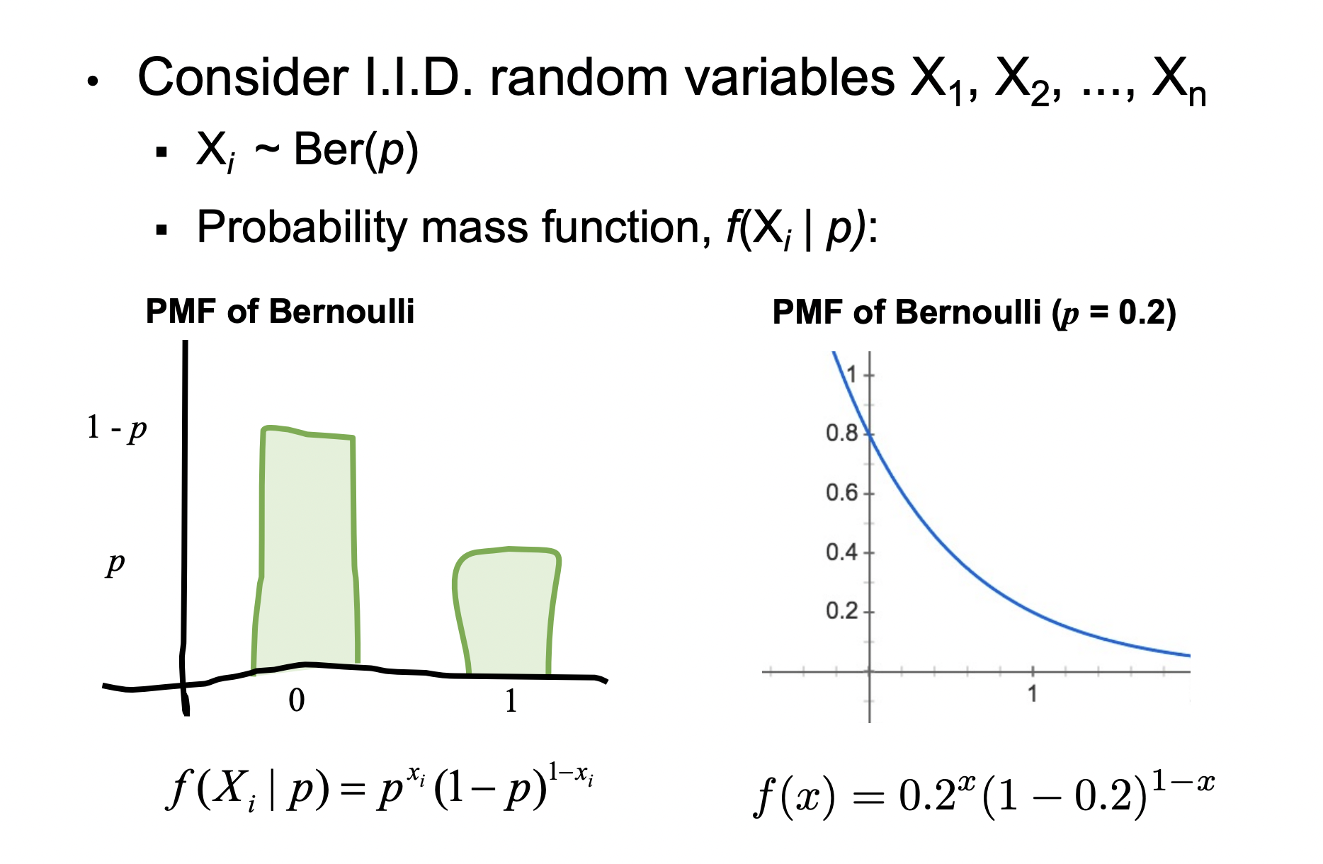
\[X \sim \operatorname{Ber}(p) \rightarrow f(X=x \mid p)=p^{x}(1-p)^{1-x}\]
A new way to choose parameters… next lecture.