Lecture 19: Bootstrapping
Before we start, one note on sampling: when we sample and plot a distribution, the distribution is not a plot of number occurrences for each sample value. No. It is probabilities for each sample value. Take below:
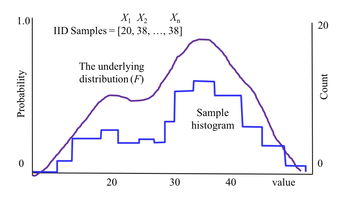
Notice on the y-axis has range of \([0,1]\).
Now let us get into sampling.
- Say we want to measure the happiness of people in Bhutan. The most accurate way to do so is to take the entire population and survey them for a score of hapiness. This will give you a complete distribution. But of course, we cannot feasibly do this. So instead, we randomly sample a small subset of the population and get their scores. Example sample: \([24,98,23,98,42,93,94,91,97,99]\).
- Now we can calculate relevant and wanted statistics about such a sample (this is called data science!) such as mean and variance. The goal is that such calculations would generalize for the entire population. Specifically, we know that the entire population would make up a true distribution if sampled entirely. So our goal here is to estimate such statistics by taking the sample’s statistics instead. We start with sample mean (denoted \(\bar{X}\)) and sample variance (denoted \(S^2\)) which are both derived on how these terms are defined for any set of data points. \[\bar{X}=\sum_{i=1}^{n} \frac{X_{i}}{n}, \quad S^{2}=\sum_{i=1}^{n} \frac{\left(X_{i}-\bar{X}\right)^{2}}{n-1}.\]
- Note: each element from the sampling set is actually just a random variable. When we draw such samples to make calculations, we of course replace them with numbers. But to work out things mathematically, we first define variables and since these take on different values at different probabilities, we just let them be random variables.
- Ok… so how well does such a sample set approximate the total population? We start by asking if our sample is biased. It isn’t and this is proved in the course notes.
- Next we ask how much my sample mean might vary relative to the true mean? Vary? sounds like “variance”. Your right. We want to calculate the variance of the mean (not the variance of the variance itself). Derivation:
\[ \begin{array}{rlr} \operatorname{Var}(\bar{X}) & =\operatorname{Var}\left(\sum_{i=1}^{n} \frac{X_{i}}{n}\right)=\left(\frac{1}{n}\right)^{2} \operatorname{Var}\left(\sum_{i=1}^{n} X_{i}\right) & \\ & =\left(\frac{1}{n}\right)^{2} \sum_{i=1}^{n} \operatorname{Var}\left(X_{i}\right)=\left(\frac{1}{n}\right)^{2} \sum_{i=1}^{n} \sigma^{2}=\left(\frac{1}{n}\right)^{2} n \sigma^{2}=\frac{\sigma^{2}}{n} & \\ & \approx \frac{S^{2}}{n} & \text { Since S is an unbiased estimate } \\ \operatorname{Std}(\bar{X}) & \approx \sqrt{\frac{S^{2}}{n}} & \text { Since Std is the square root of } \end{array} \] \[\begin{array}{rlr}\operatorname{Var}(\bar{X}) & =\operatorname{Var}\left(\sum_{i=1}^{n} \frac{X_{i}}{n}\right)=\left(\frac{1}{n}\right)^{2} \operatorname{Var}\left(\sum_{i=1}^{n} X_{i}\right) & \\ & =\left(\frac{1}{n}\right)^{2} \sum_{i=1}^{n} \operatorname{Var}\left(X_{i}\right)=\left(\frac{1}{n}\right)^{2} \sum_{i=1}^{n} \sigma^{2}=\left(\frac{1}{n}\right)^{2} n \sigma^{2}=\frac{\sigma^{2}}{n} & \\ & \approx \frac{S^{2}}{n} & \text { Since S is an unbiased estimate } \\ \operatorname{Std}(\bar{X}) & \approx \sqrt{\frac{S^{2}}{n}} & \text { Since Std is the square root of Var }\end{array}.\]
- This last part (\(\operatorname{Std}(\bar{X}) \approx \sqrt{\frac{S^{2}}{n}}\)) has a special name: standard error: and its how you report uncertainty of estimates of means.
- Applied example: Let’s say we calculate the our sample of happiness has \(n = 200\) people. The sample mean is \(\bar{X}=83\) and the sample variance is \(S^2 = 450\). We can now calculate the standard error of our estimate of the mean to be \(1.5\). When we report our results we will say that the average happiness score in Bhutan is \(83 ± 1.5\) with variance \(450\). And done!
- See how we give a “confidence interval” in how well our approximation was for the true distribution (i.e. the distribution you’d get if you sampled the entire population). And so in this light, the standard error allows us to quantify our belief bounds in the sample mean representing an approximation of the true distribution.
Bootstrapping
We now discuss an important algorithm (invented at Stanford!). It is a newly invented statistical technique that allows us to understand distributions better and also allows us to calculate p-values: the probability that a scientific claim is incorrect.
- It was invented as a consequence of using computing to capture insights in probability theory. Specifically, the key insight here is that if we had access to the underlying distribution of our samples (i.e. its PDF/PMF), then we can answer any question we might have regarding the accuracy of our statistics we calculated from our original sample (e.g. how close our sample mean is to the true mean). But why so? Well… it goes like this:
- What if we want to know the probability that the true variance is within a certain range of the number we calculated? If you knew the underlying distribution, \(F\), you could simply repeat the experiment of drawing a sample of size \(n\) from \(F\) (i.e. a sample set consisting of \(n\) items), calculate the sample variance from our new sample and test what portion fell within a certain range.
- Side note: when we “sample”… we are not referring to a singular number (unless \(n=1\)). But rather we refer to a set of size \(n\) consisting of \(n\) drawings from the distribution.
- What if we want to know the probability that the true variance is within a certain range of the number we calculated? If you knew the underlying distribution, \(F\), you could simply repeat the experiment of drawing a sample of size \(n\) from \(F\) (i.e. a sample set consisting of \(n\) items), calculate the sample variance from our new sample and test what portion fell within a certain range.
- But of course we aren’t really going to be given \(F\), the distribution function. Instead, we’d need to estimate that as well which we can do in a similar fashion: the best estimate that we can get for \(F\) is from our sample itself! The simplest way to estimate \(F\) (and the one we will use in this class) is to assume that the \(P(X = k)\) is simply the fraction of times that k showed up in the sample. And this defines the PMF of our estimate \(\hat{F}\) of \(F\).
Pseudocode:
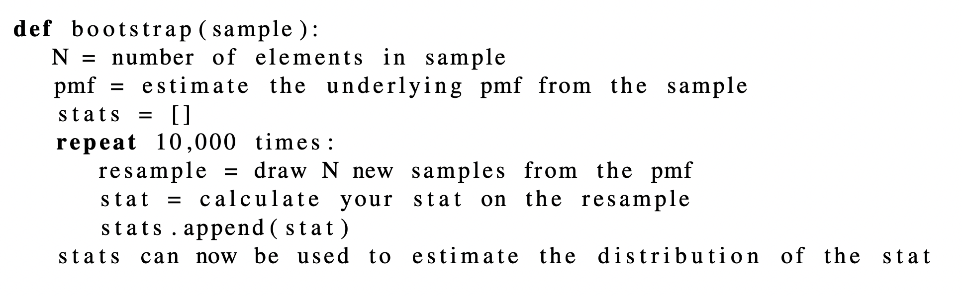
Here is the idea:
- We draw our initial sample from the population. For example, get the hapiness scores of 200 people from Bhutan.
- Plot these scores as a histogram with probabilities for each value. This is our initial sample distribution. But we want to make it more accurate. Bootstrapping gives us a way to do this (specifically to estimate the true distribution). Here is what we do next.
- We loop a certain amount of times. Each time in the loop, we draw \(n\) samples from the histogram distrubution we just created (we are sampling from this distribution). This gives you a set of \(n\) elements. Now we can calculate the relavant statistic (e.g. mean, variance) we want from this set and append this to a list.
- After the loop, we should have a new set of statistics. We can plot these and this forms our new distribution.
Side note: we don’t actually end up with a whole new distribution in the same unit as the true distribution. Instead, we calculate this in the context of a relavant statistic we want for each new statistic. For example, take variance. Bootstrapping leaves us with a whole new distribution for the variance which aims to estimate the true underlying distribution’s variance.
- Key insight: say we want to estimate the true variance of happiness scores in Bootan (pun intended here). We take 200 people from the population and plot out a distribution of hapiness scores. This gives us a “fake”/estimate of the true underlying distribution (let’s call it \(\hat{f}\)). Now we can go and calculate the variance directly outright from here by drawing \(n\) elements from \(\hat{f}\) but that wouldn’t be that accurate. Instead, what we do is run a loop and get tons of samples of size \(n\) and calculate the sample variance for each of these sets. Now these calculations itself form a set. And now to get what we wanted, we simply take the variance of this master set which accruately measures the true variance. Voila!
Side note: in Python, to sample from a histogram (i.e. the initial 200 people you observed), use code from the official lecture slide deck.
The key point about bootstrapping is that it allows us to calculate the accuracy of such statistics.
Also note: we just keep on resampling from the data we are given (not just some \(n\) subset).
Summary: say we want to measure a statistic about the general population. We of course cannot survey the entire population so instead we take a sample of size \(n\). Then, bootstrapping allows us to estimate what the true distribution (i.e. if the whole population had indeed been sampled) is by resampling. Specifically, the algorithm goes like this: 1. take your initial sample from the population of size \(n\). 2. Create a loop of 10,000 or greater times. At each iteration, draw a sample, of size \(n\) from the initial sample. 3. Calculate your statistic you want on this subset sample. Append it to a master list. 4. After the loop, calculate the statistic on this master list itself. This is you answer.