Lecture 16 - Beta
Date of when lecture was given: 02/11/22.
We now begin discussion of an entire new unit: uncertainty theory. We will have a meta discussion about probabilities: what happens when there is uncertainty in our probabilities themselves?! We need some sort of measure to quantify uncertainty. Unless you have been sleeping under a rock this entire quarter, this should scream: “probability is the measure of uncertainty”. Yes. Yes, that is right. We will use probabilities to measure the uncertainty of other probabilities (via random variables). This is the most theoretical and therefore most mathematical part of the course.
Probability as a random variable
Example: You ask about the probability of rain tomorrow. Person A: My leg itches when it rains and its kind of itchy…. Uh, \(p = .80\). Person B: I have done precise, complex calculations and have seen 10,451 days like tomorrow… \(p = 0.80\). What is the difference between the two estimates?
Example: you are buying an item on Amazon and are deciding between two different models. The first model has all 5-star ratings! Woohoo! And the second model has an average of 4.3 stars. Easy decision right? Wrong. It turns out the 5-star rating has only 5 reviewers whereas the second model has over thousands of reviewers. Which one do you choose now? This type of uncertainty in our belief for each item model is what we will discuss today.
Remark: Until now probabilities have just been numbers in the range 0 to 1. However, if we have uncertainty about our probability, it would make sense to represent our probabilities as random variables (and thus articulate the relative likelihood of our belief).
We introduce the beta random variable in this light via annotated example.
Beta random variable
Say we have some coin and we want to know the probability, \(p\), that it will turn up as heads (the age old question). We flip the coin a total of \(n+m\) times where \(n\) is the number of heads and \(m\) is the number of tails (so \(n+m\) is all flips). And so we have
\[p=\frac{n}{n+m}.\]
But is this really true? What if we only flip the coin 3 times total? We might get something like \(p \approx 0.33333\). Are we really certainly about our belief in this probability? Can you guess what I am hinting it (uncertainty in our belief!)? This number (\(p=\frac{n}{n+m}\)) doesn’t capture our uncertainty about \(p\) itself. So just like anything with uncertainty, we propose to capture such semantics via a distribution for the values that \(p\) can take on.
Recall that we defined a random variable as something that can take on different values at different probabilities. To formalize the idea that we want a distribution for \(p\), we are going to use a random variable \(X\) to represent the probability of the coin coming up heads. And so we can define probabilities that \(X\) takes on a certain probability. Probability is a continious measure and has a range (support) between 0 and 1.
And so without any prior belief in what \(X\) can be, we assume that each value that \(X\) can take on is equally likely (that is, we assume \(X\) can take on any probability at an equally likely rate). For this reason, we start by saying
\[X \sim U n i(0,1).\]
Now how do we “update our beliefs about a random variable/probability”?! You got it. Bayes’ theorem. So we wil condition on another random variable that represents the new observations. For the Beta distribution, we condition on Binomials (take a moment to understand this: you are conditioning on an entirely separate distribution… how you obtain that distribution can be through frequentist experiment trials or be given the distribution predeterminedly).
Say we start to flip the coin a few times now and we want to update our beliefs (probabilities) for \(X\). This is actually a whole experiment in it of itself. And so let \(N\) be a random variable that represents the number of heads that can come up, given that the coin flips are independent. So we define our binomial. But of course, we need to plug in a parameter \(p\) for our binomial so we actually condition on \(X\) itself first. That is,
\[(N \mid X) \sim \operatorname{Bin}(n+m, x).\]
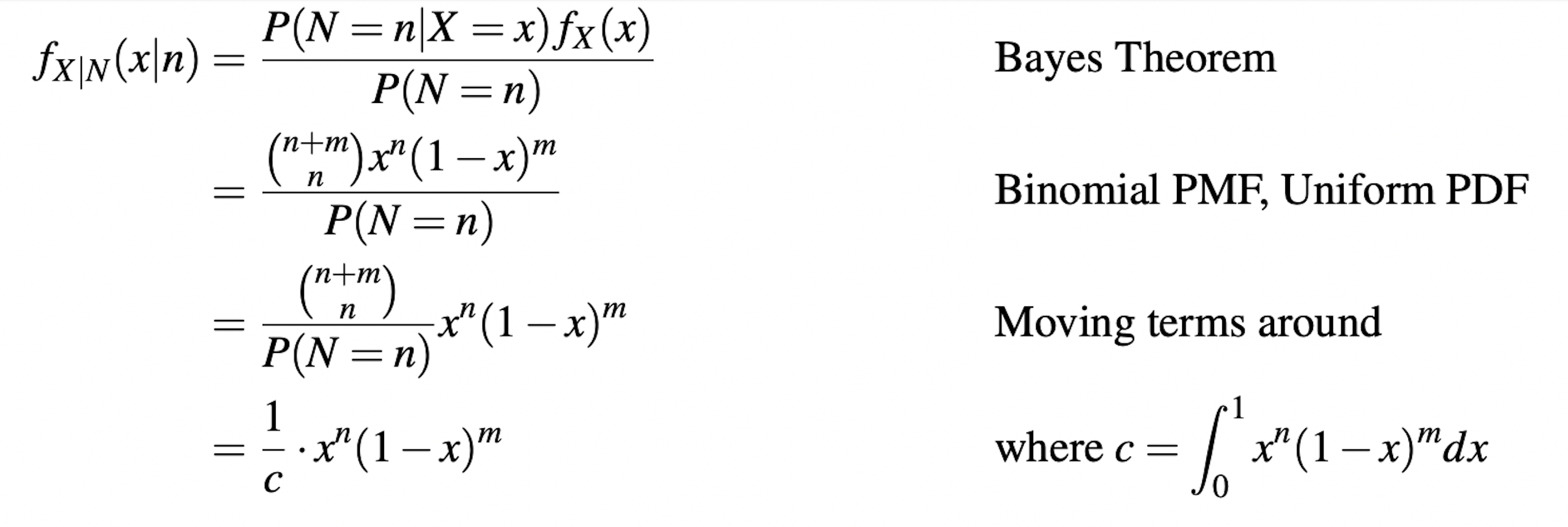
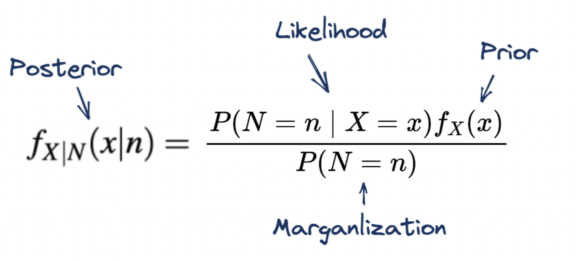
Recall that the little \(x\) is a probability. So we now apply Bayes’ theorem to update our belief in \(X\) given the new Binomial distribution for \(X\) (specifically we want to calculate the PDF distribution for \(X\) given \(N\)):
Now notice one specific thing. Remember that each component of Bayes’ theorem has a name:
Summary
So in summary, we stated that we might have uncertainty in our beliefs (probabilities) themselves. Thus, we decided to represent probability as a random variable, \(X\). Now we aimed to find a parametric distribution for the random variable. Initially, we started with a uniform distribution: \(X \sim U n i(0,1)\) where the value that \(X\) can take on is equally likely. But of course, we want to update such a belief for \(X\) given some observed experimental trials (or expert knowledge). So we use conditional probability in the form of Bayes’ theorem. In this case, we condition on a Binomial RV, \(N\) (i.e. coin flips experiment).
\[ f_{X \mid N}(x \mid n)=\frac{P(N=n \mid X=x) f_{X}(x)}{P(N=n)} \]
But realize that we have a prior! A lot of times we can just keep this as a uniform because we may not know any previous knowledge beforehand. But sometimes we do. For example, we may know that a certain drug is likely to work to a certain degree based on expert knowledge. And to incorporate such knowledge of this in the calculation, we can define the prior as such. Notice that the prior is also an RV PDF (i.e. \(f_{X}(x)\)) which represents the initial beliefs in our probabilities (so in some way this is recursion but it really isn’t because we are usually given such information). That is, we incorporate such domain knowledge via a probability density function which represents the beliefs in the probabilitied for \(X\) initially (“prior information”). This is the thing we are updating! To this in it of itself can be any RV that has range \([0,1]\) which leaves us with either a beta RV and uniform RV. And so if we have some prior non-uniform belief, we must use a beta to represent that belief! So yes, We are using a beta RV to derive the PDF for the beta. But don’t worry, this isn’t recursion because you’d usually be given such a beta or at least the information needed to describe and therefore denote it (i.e. through expert domain knowledge or repeated experimentation). Note that such a property is called a conjugacy: we are deriving the posterior from the same distribution family in the prior.
Ok… so we have the idea and intuition down: we need our prior to be a beta. But we haven’t even given the derivation for a beta yet. We mentioned that this information is gained by things like expert knowledge or repeated trials. We will talk about deriving the beta for the latter (the former is usually given).
We flip a fair coin defined as X ~ Uni(0, 1) prior over probability, and observe: \(n\) “successes” and \(m\) “failures”. By the Binomial distribution, our new belief in \(X\) is \[ f_{X}(x)=\frac{1}{c} \cdot x^{n}(1-x)^{m}. \] where \(c=\int_{0}^{1} x^{n}(1-x)^{m}\). And so plugging this in as our prior in the original Bayes’ derivation above, we have \[ \begin{aligned} f(X=x \mid N=n) &=\frac{P(N=n \mid X=x) f(X=x)}{P(N=n)} \\ &=\frac{\left(\begin{array}{c} n+m \\ n \end{array}\right) x^{n}(1-x)^{m} f(X=x)}{P(N=n)} \\ &=\frac{\left(\begin{array}{c} n+m \\ n \end{array}\right) x^{n}(1-x)^{m} \frac{1}{B(a, b)} x^{a-1}(1-x)^{b-1}}{P(N=n)} \\ &=K_{1} \cdot\left(\begin{array}{c} n+m \\ n \end{array}\right) x^{n}(1-x)^{m} \frac{1}{B(a, b)} x^{a-1}(1-x)^{b-1} \\ &=K_{3} \cdot x^{n}(1-x)^{m} x^{a-1}(1-x)^{b-1} \\ &=K_{3} \cdot x^{n+a-1}(1-x)^{m+b-1} \\ X \mid N & \sim \operatorname{Beta}(n+a, m+b) \end{aligned}. \]
PDF: \[ f(x)=B \cdot x^{a-1} \cdot(1-x)^{b-1}. \]
There you have it folks: the beta random variable derived by conditioning a uniform on a Binomial! See here and here.
Summary: ok… now a real short and sweet summary. We want a random variable to measure our beliefs in the some binomially distributed process (e.g. coin flips). We start by defining \(X\) as a uniform: \(X ~ Uni(0, 1)\). Now we perform some experiment (i.e. flipping the coin some number of times) which gives us a binomial RV, \(N\). We condition \(X\) on \(N\) to update our beliefs about \(X\): \[ f(X=x \mid N=n)=\frac{P(N=n \mid X=x) f(X=x)}{P(N=n)} \]
More notes
- Random variable for measuring probabilities
- So you have a distribution of probabilities
- Support is 0 to 1.
- Probability… so it is continuous
- The input parameters are like a Binomial experiment. For example, we flip a coin 10 times and it comes up heads 7/10 times and tails 3/10 times. So what is our distribution of probabilities that such a random variable can take on? Well, certainly given the observed data, we see that the most likely probability should be 7/10.
- So we now have a distribution of probabilities for each of the probabilities that the coin can take on (and thus articulate the relative likelihood of our belief).
Frequentist vs. bayesian
Two schools of thought and it boils down to a component of an equation.
- In the coin flips example, we can simulate billions of coin flips instantly and approach the problem from a frequentist point of view (\(\frac{m}{m+n}\)). However…
- We might want to assign a Beta random variable that represents the probability of a medical drug working. We cannot simulate this on billions of people. So we have to use our expert domain prior knowledge about the world somehow. This is the Bayesian world view.
- See
50:00of lecture 16.
Take this example:
When we use beta as a prior, we don’t need to do the above derivation because the posterior is from the same distribution. So all we need to do is add the number of successes and number of failures to our prior parameters for beta and we get the newly defined posterior. The derivation works out to be \(\operatorname{Beta}(a+h, b+t)\) where \(a\) and \(b\) are the original parameters and \(h\) and \(t\) are the updated number of successes and failures.
Application: You might be asked to calculate the updated belief in \(X\), already defined as a beta of the form \(\operatorname{Beta}(a, b)\) given \(h+t\) new trials where \(h\) is number of new successes and \(t\) is number of new failures. So the new RV is just \(\operatorname{Beta}(a+h, b+t)\). Derivation is given in course reader but it is just a repeated application of Bayes’ theorem.
In our original derivation for the beta, we conditioned \(X \sim Uni(0, 1)\) on \((N \mid X) \sim \operatorname{Bin}(n+m, x)\) which gave us the PDF for a beta: \[f(X=x)=\left\{\begin{array}{ll}\frac{1}{B(a, b)} x^{a-1}(1-x)^{b-1} & \text { if } 0<x<1 \\ 0 & \text { otherwise }\end{array} \quad\right.$ where $B(a, b)=\int_{0}^{1} x^{a-1}(1-x)^{b-1} d x\]
Now we can continiously update our belief on \(X\) with other RVs as priors but if that new prior happens to be a beta… our update is very simple!: \[\operatorname{Beta}(a, b) \rightarrow \operatorname{Beta}(a+h, b+t). \]
Note: the original derivation for the beta was done by updating a uniform conditioned on a binomial. Here we condition a beta on a binomial (and so our prior is a beta and we actually end up with another beta which is our posterior).
Another note: if the posterior is the same as the prior (i.e. conjugacy), you should realize that all you are doing is updating the parameters.
Ok… back to the lecture at 50:00:
- Can use laplace prior instead of uniform to prevent probability being 0. Can be nicer in code.
- Imagine a scenario where we need to decide betwe en two drugs to give to patients. Let us say we have two beta distributions that represent the probabilities that each drug is a success. We can use a greedy approach that is referred to as Thompson sampling. It goes like this. Sample from your first beta distribution (giving a probability). Now sample from your second beta distribution (giving you another probability). You should choose the drug whose sample was a higher probability. Why? Because the confidence is higher in that drug (see around
1:15for a more detailed explanation).- This allows us to make good decisions “under uncertainty”.
- This has a whole host of applications such as in RL for game-playing agents (which path should I take in chess?).
- A lot of these algorithms though use similar, but more complex RL algorithms.