Lecture 15: General Inference
Roadmap of unit
- We started out by specifying the joint distribution which gave us all of the information we would ever need about jointly distributed multiple random variables.
- We then developed intuition for conditional probability between a whole mixture of random variables (e.g. Bayes’ rules).
- We then came up with questions we’d like to answer related to conditional probability. We call these questions “inference”.
- However, as our system of random variables grew larger, the joint becomes computationally intractable to specify.
- So instead, we developed probablistic graphical models (Bayesian networks) which is a graphical model of causalities (nodes are RVs and edges imply causality/conditionallity). Because of dependence between the RVs, this greatly reduces the number of calculations we need for general inference questions… to get the probability of a particular node/RV taking on a value, we only need its parent probabilities to get this value (i.e. conditioned on the parents).
- But… we still don’t know how to exactly get these values from the graphs (i.e. generally infer from the graph). Today, we learn that.
- Don’t know how to solve probability questions from Bayesian networks.
- Many techniques for doing so but main one today that we’ll learn is called “sampling”.
- We will sample from this hypothetical joint distribution that we are modelling using the Bayesian network to answer general probability questions.
- Covariance: how much they differ from the mean
- Correlation does not equal causation
- Covariance looks for linear relationship.
- So covariance/correlation doesn’t tell us everything: some RV’s might be nonlinearlly correlated.
Small note example: take the following Bayesian network:
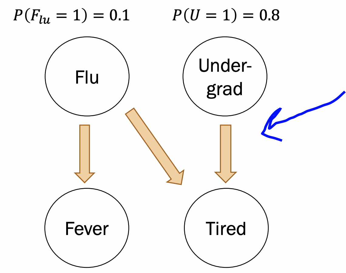
Notice that
\[ P\left(F_{e}=0 \mid U=1, F_{L}=0\right) = P\left(F_{e}=0 \mid F_{L} = 0 \right) \]
because fever has no dependence on undergrad. Recall definition of independence: \(P(E|F) = P(E)\). This is called the “independence assumption”.
Rejection sampling
So how we actually compute inference questions from Bayesian networks?
We can start with \[ P\left(F_{l u}=1 \mid U=1, T=1\right) \]
which is chain rule of conditional probability. However, the denominator would require a marganlization of tons of RV’s potentially. Let us come up with a more intuitive method for answering any inference question we may come upon in a systematic way. We call it rejection sampling because it works by sampling and rejecting the faulty samples.
Steps: - Step 0: Have a fully specified Bayesian network layed out. - Step 1: sample a ton! Remember sampling: given some random variable distribution, if we were to randomly take one value from that distribution, we get a sample (of course the value we get is dependent on the probabilities of that random variable taking on that value: it is inverse). So we essentially do this for all nodes (RVs) in the network. This gives us a joint sample. - Step 2: so how do we compute conditional probability questions? Well, now that we have a bunch of samples, we reject the faulty ones. What do we mean? You can imagine we have a bunch of samples:
# [Flu, Undergrad, Fever, Tired]
[0,1,1,1]
[0,1,0,0]
[1,0,1,0]
[0,0,0,0]
.
.
.
[1,1,1,1]
say we want \(P(Flu = 1 | U = 1)\). We can loop through all samples, then throw out every sample not consistent with the observation (that is, \(U=1\)). So if we loop through all our samples and it doesn’t have a \(1\) in the index corresponding to \(U\), we throw (reject) it out. This will give you a subset of the samples that are all consistent with the observation. Now loop through this subset and count the number of times the index corresponding to \(Flu\) has a \(1\). Divide this count by the length of this sample subset (the subset whose elements are samples consistent with the observation).
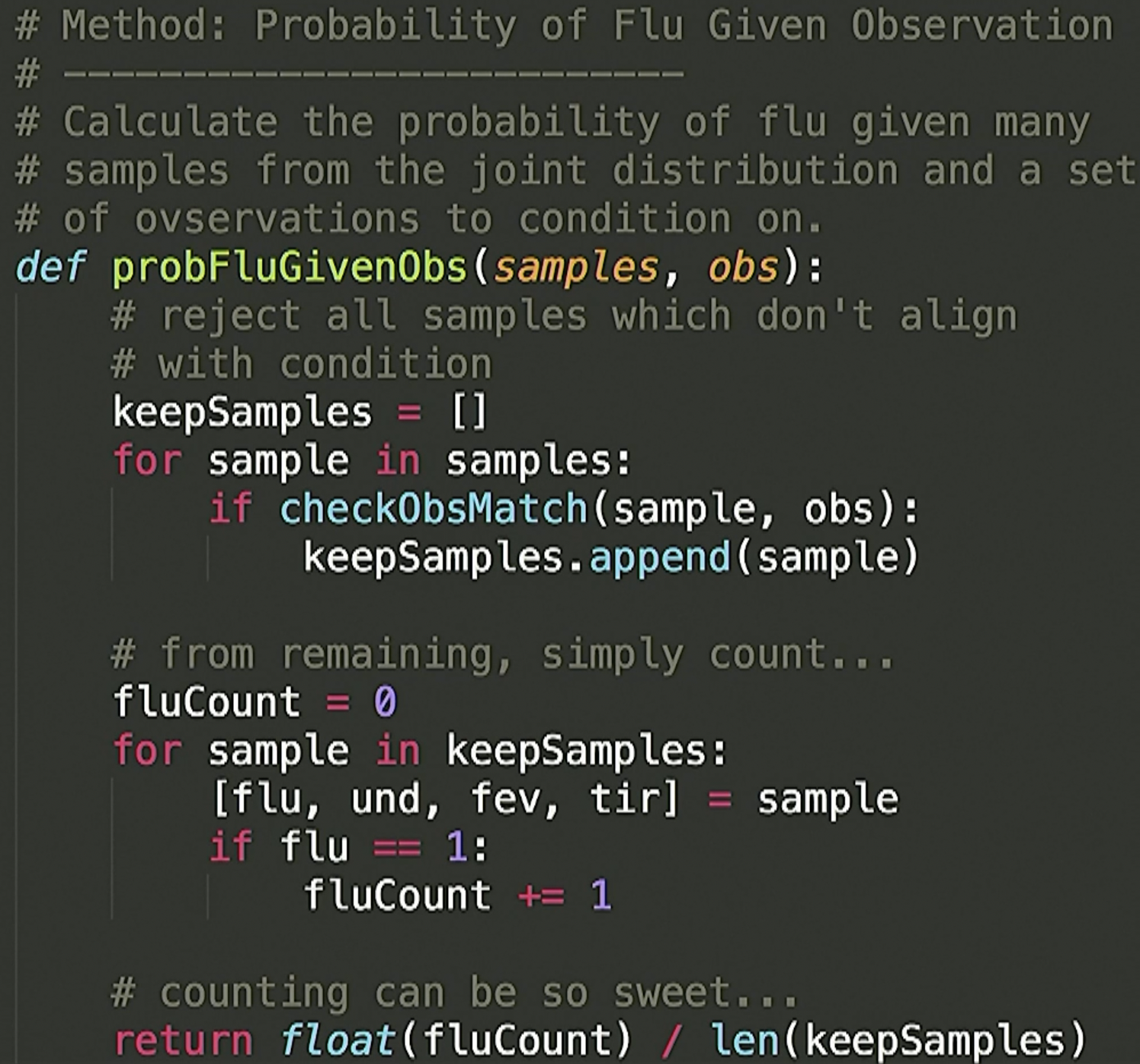
Pseudcode: - Step 0: Have a fully specified Bayesian network layed out. - Step 1: sample a ton! - Step 2: collect subset of samples consistent with observation (thing you are conditioning) - Step 3: loop through this subset and count number of times the thing you want the probability of is present in the sample. - Step 4: Divide this count by the length of this sample subset (the subset whose elements are samples consistent with the observation).
Limitations
Ahh… rejection sampling seems to good! However, we only worked with discrete RV’s. Sometimes we might have a continious RV in the mix and rejecting such a sample with a continious RV is a different task than if the numbers jut match. This is because the probability of a CRV taking on an exact value is 0. Thus, no samples will match exactly and you’d reject all of them leading to division by 0.
So what is the solution? Another algorithm we can use is called Markov Chain Monte Carlo (MCMC)!
Welp… we learn that in a different class.