Lecture 14 - Modeling
- Inference is when you ask conditional probability questions about a joint distriubtion.
- We also learned how to update our beliefs about a random variable given some result from another random variable (see eye test lecture example).
- Posterior belief.
- Remember that you cannot have a probability/posterior of a random variable itself: \(P(X)\) makes no sense (this is object/function). Instead, you need it to be an event: when your RV takes on a value. So if you want to update a discrete random variable distribution conditioned on another random variable taking on a particular value (i.e. the student got the answer correct), you need to update every event possible for that random variable. In other words, you need to apply Bayes’ to all of \(P(X=x_1)...P(X=x_n)\). These posterior beliefs make up your posterior distribution.
- Normalize: sum up all the possible beliefs (sum up \(P(X=x_1)...P(X=x_n)\)) to get the normalization constant for the denominator of the Bayes’ theorem formula:
- This is necessary when you are updating your belief about all possible events for the random variable. \[\begin{aligned} P(A=a \mid Y=0) &=\frac{P(Y=0 \mid A=a) P(A=a)}{P(Y=0)} \\ &=\frac{P(Y=0 \mid A=a) P(A=a)}{\sum_{a} P(Y=0, A=a)} \\ &=\frac{P(Y=0 \mid A=a) P(A=a)}{\sum_{a} P(Y=0 \mid A=a) P(A=a)} \end{aligned}\]
- Called normalize because makes all posterior beliefs correctly sum to 1.
New topics: 1. Probabilistic modeling 2. Correlation 3. Independence with random variables
Modeling
- Inference is when you ask conditional probability questions about a joint distriubtion.
- In WebMD, we might want to know what \(P(X=1 | U=1)\) is where \(X=1\) means you have a virus and \(U=1\) means you are an undergraduate student (or could be a symptom etc.). Asking these questions is inference.
- Ideally, we can be given a joint distribution and answer any question we like. But as we know, we cannot do that cuz the size of the distribution increases rapidly and becomes an \(np\)-hard problem (computationally intractable). So we need better “models” for the joint.
- One way to do this is via a graph:
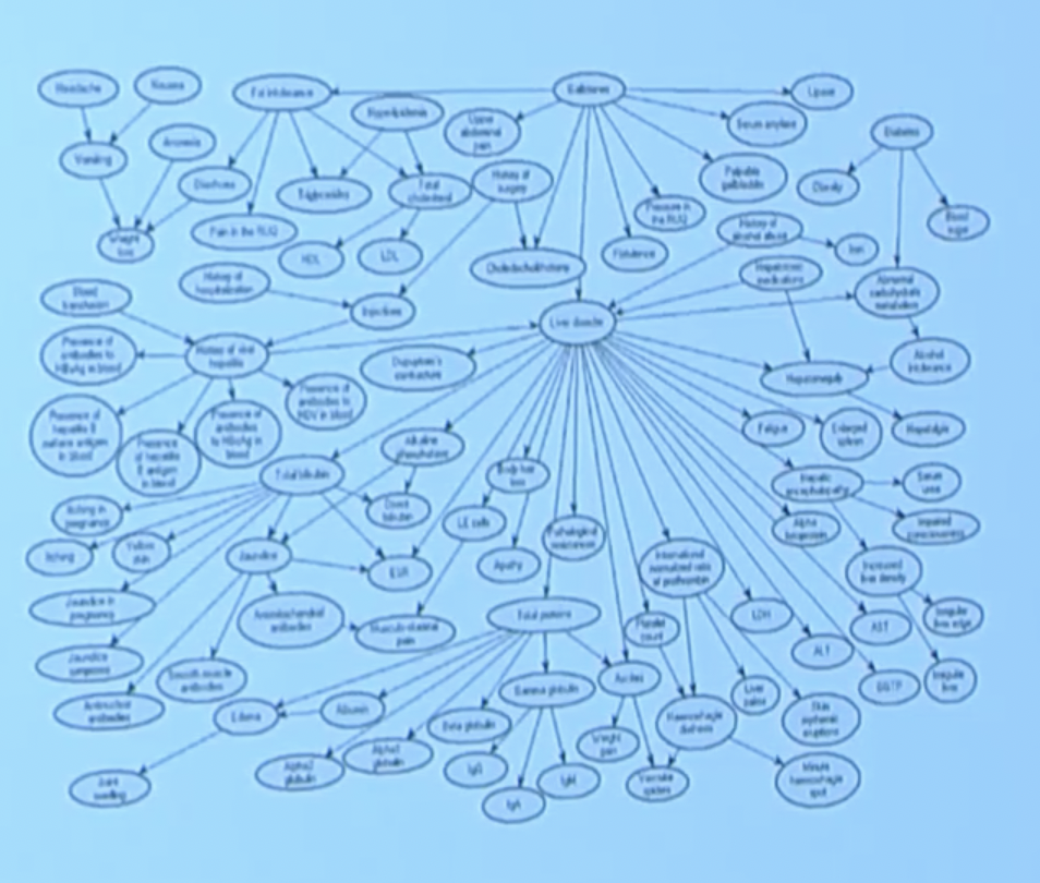
- Using the nodes and edges, you can start to calculate conditional probability questions.
- These are called “Bayesian networks”.
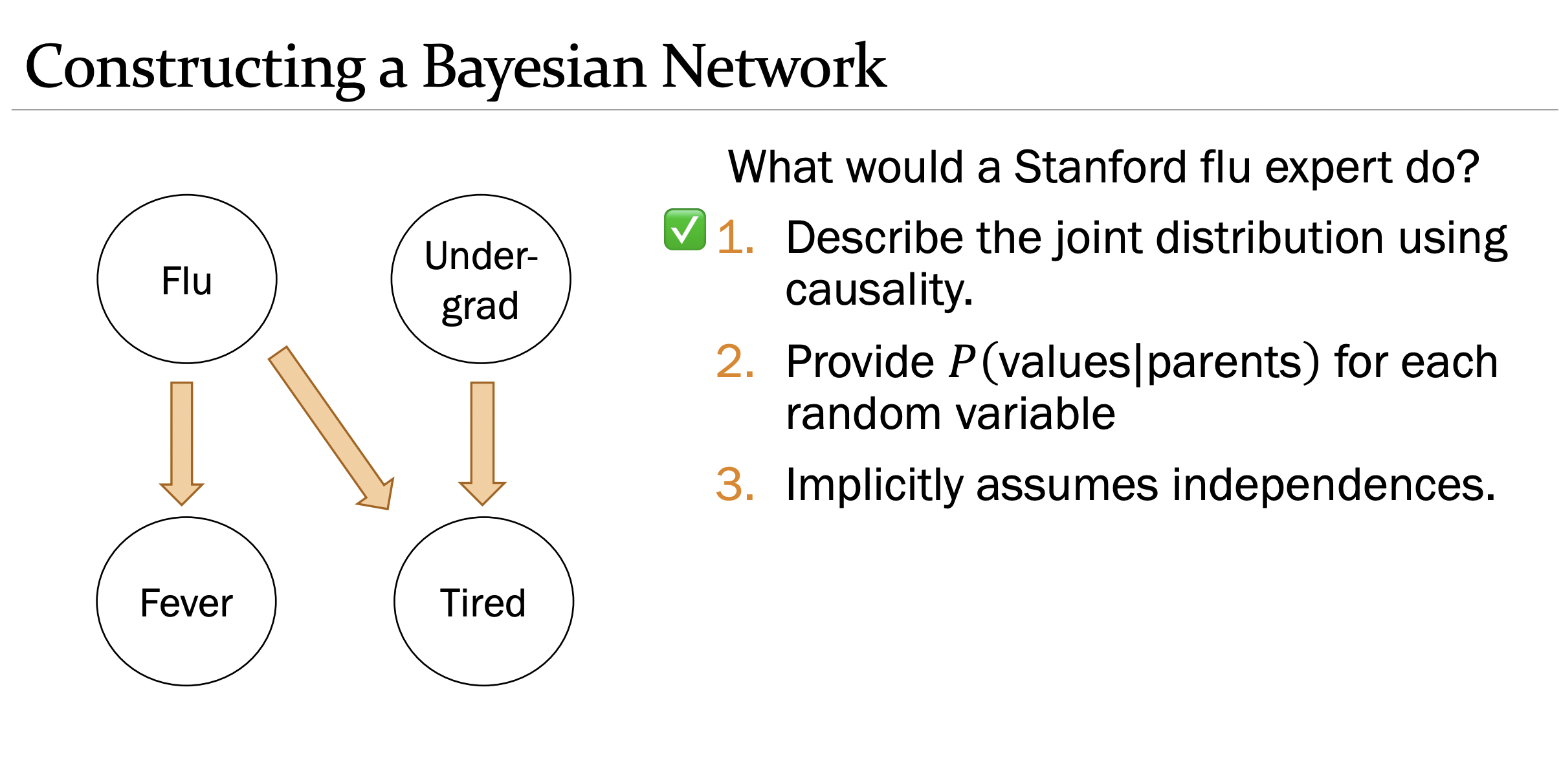
- The artform of making a BN is describing the hypothetical joint distribution using causality. You might have a node such as “undergrad bernoulli” and another “tired ernoulli”. We know being an undergrad causes you to be tired. This is how we’d form our model.
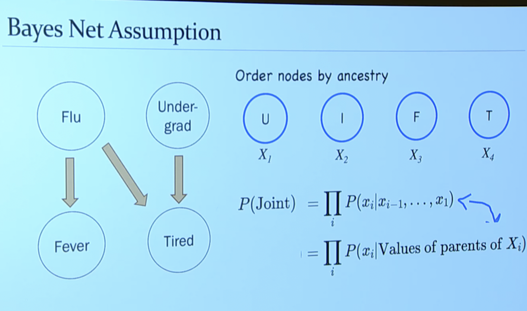
- Once we have the directed graph, we can answer inference (conditional probability questions). If you think about it, it makes to condition a random variable event on its parents (e.g. prob. tired conditioned on being an undergrad). \[ \prod P\left(x_{i} \mid \text { Values of parents of } X_{i}\right). \]
- So to estimate the full joint, we need to:
- Construct directed graph where each node is a random variable and each edge represents causality (conditioning).
- Then, to approximate the joint, instead of filling in a table of all possible combinations, we’d just need to calculate the values for each node (but this is easier because each node/RV is conditioned on its parents!).
- Notes:
- One constraint is that the graphs must be acyclic meaning you cannot have a directed edge pointing in both ways. This makes sense because you cannot have a conditional going in both directions (only one thing can cause another thing). This is an assumption we make to make the math fit into the probabilistic framework. Helpful slides:
Independence
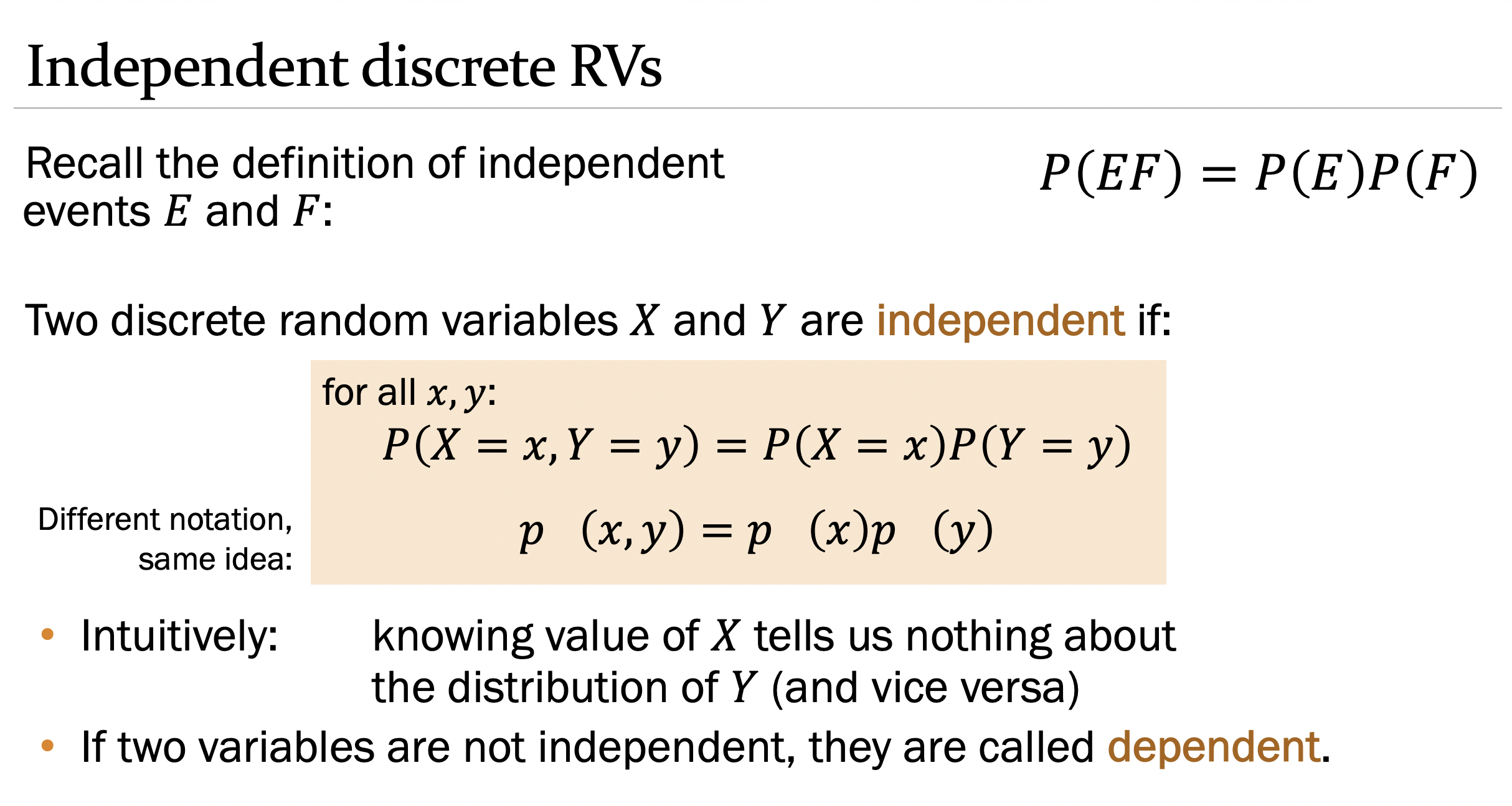
- For RV’s to be independent, all possible events between the two must be independent.
How do we measure independence? Covariance!
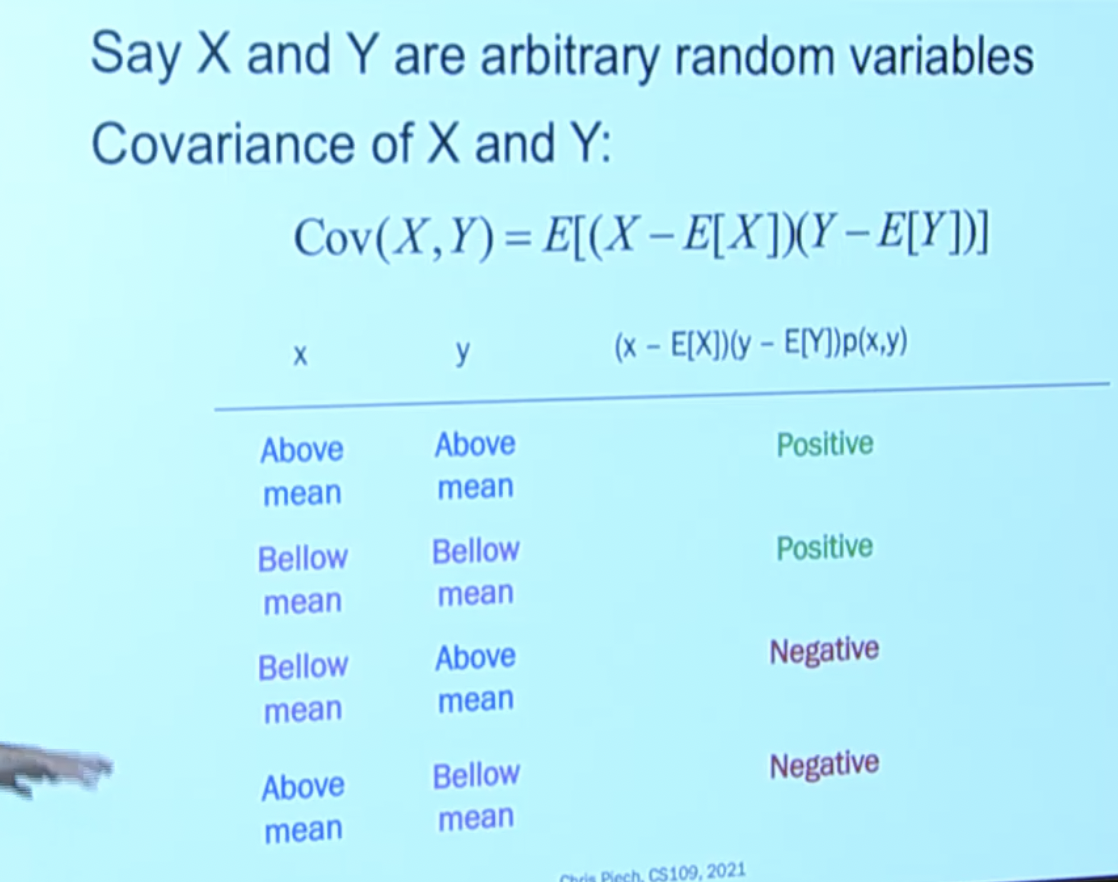
Covariance: how do we measure how related (how much the vary together) two random variables are? We do it with a metric called covariance: \[ \begin{aligned} \operatorname{Cov}(X, Y) &=E[X Y-E[X] Y-X E[Y]+E[Y] E[X]] \\ &=E[X Y]-E[X] E[Y]-E[X] E[Y]+E[X] E[Y] \\ &=E[X Y]-E[X] E[Y] \end{aligned} \]
If \(X\) and \(Y\) are independent, then \(\operatorname{Cov}(X, Y)=0\). But \(\operatorname{Cov}(X, Y)=0\) doesn’t necessarily imply independence.
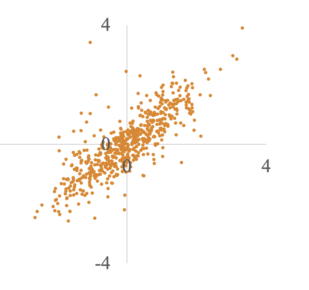
Positive covariance (positive linearly correlated)
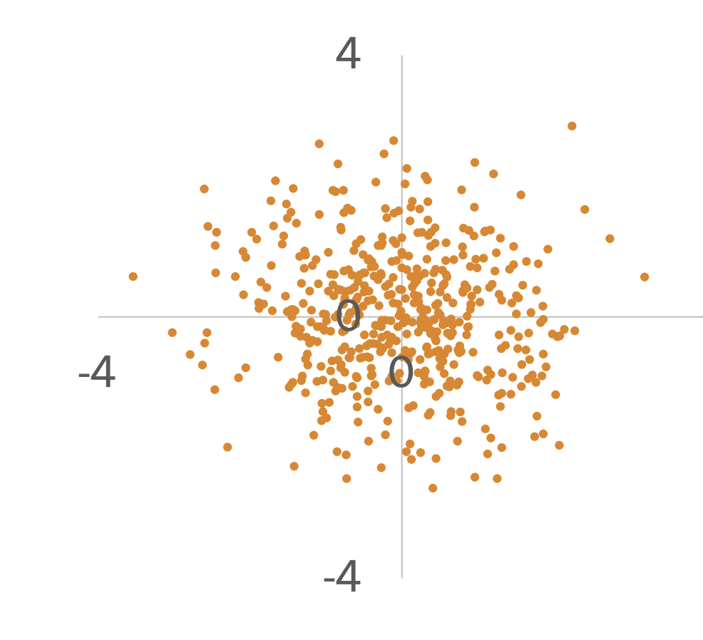
Zero covariance
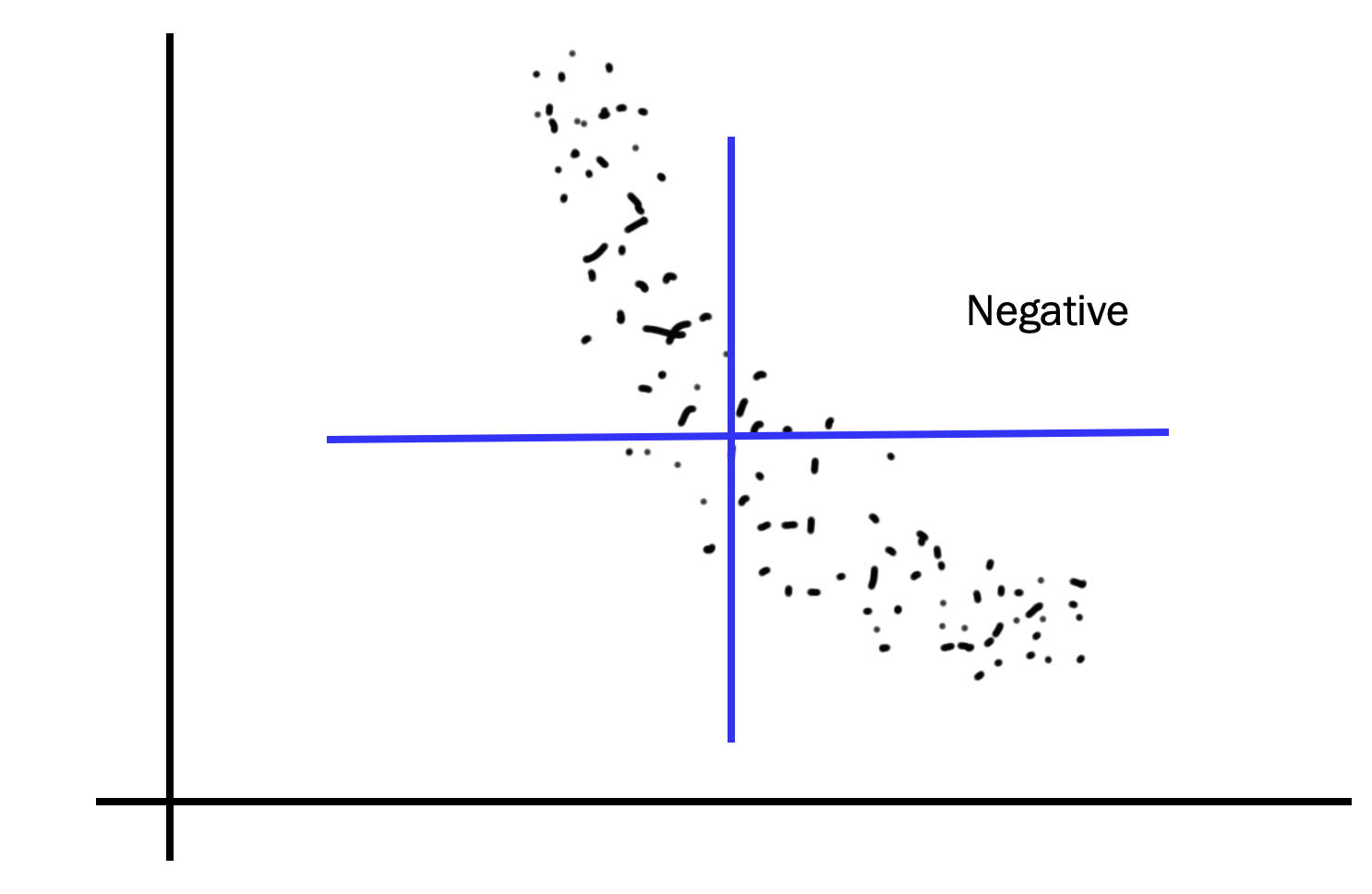
- Negative covariance
Correlation
You might be thinking… hmm covariance doesn’t really have a “unit” per say. What does “covariance” even mean besides being just a metric? So people came up with correlation:
Measures “linearity”
Covariance is a quantitative measurement of the relationship between two variables. Correlation between 2 RVs, \(\rho(X, Y)\) is covariance of the two variables normalized by the variance of each variable. This normalization cancels units out and normalizes the measure so that it is always in the range \([0,1]\) : \[ \rho(X, Y)=\frac{\operatorname{Cov}(X, Y)}{\sqrt{\operatorname{Var}(X) \operatorname{Var}(Y)}} \] Correlation measure linearity between \(X\) and \(Y\). \[ \begin{array}{ll} \rho(X, Y)=1 & Y=a X+b \text { where } a=\sigma_{y} / \sigma_{x} \\ \rho(X, Y)=-1 & Y=a X+b \text { where } a=-\sigma_{y} / \sigma_{x} \\ \rho(X, Y)=0 & \text { absence of linear relationship } \end{array} \] If \(\rho(X, Y)=0\) we say that \(X\) and \(Y\) are “uncorrelated.” If two varaibles are independent, then their correlation will be 0 . However, it doesn’t go the other way. A correlation of 0 does not imply independence.
Given historical data, we can use correlation and covariance to figure out how to construct our Bayesian networks!