Lecture 13: Inference part II
Bayes’ theorem with discrete RV’s is easy: it is just a table with a bunch of lookups. The real complexity arises when you have a continious random variable in the mix because now you are dealing with densities instead of probabilities. We will explore that in the next lecture.
We will use the following as a guiding example:
- Question: At birth, girl elephant weights are distributed as a Gaussian with mean \(160 \mathrm{~kg}\), and standard deviation \(7 \mathrm{~kg}\). At birth, boy elephant weights are distributed as a Gaussian with mean \(165 \mathrm{~kg}\), and standard deviation of \(3 \mathrm{~kg}\). All you know about a newborn elephant is that it is \(163 \mathrm{~kg}\). What is the probability that it is a girl?
The initial set up using Bayes’ would be: Let \(G\) be the event that the elephant is a girl (discrete Bernoulli indicator). Let \(X\) be the event that the elephant weighs \(163\) kg (continious Gaussian)
\[ P=(G=1|X=163) = \frac{P(X=163 | G = 1)P(G=1)}{P(X=163)} \]
Now notice: anything that involves \(P(X=x)\) taking on a specific value \(x\), we have a problem: a continious random variable cannot take on a specific value! So we must use a trick.
We need some width under the curve to multiply the density by and we called it \(\epsilon\). Luckily, by the Bayes’ formula, were gonna be able to cancel them out:
\[P(N=n \mid X=x)=\frac{P(X=x \mid N=n) P(N=n)}{P(X=x)},\] \[P(N=n \mid X=x)=\frac{f(X=x \mid N=n) \cdot \epsilon \cdot P(N=n)}{f(X=x) \cdot \epsilon},\] \[P(N=n \mid X=x)=\frac{f(X=x \mid N=n) \cdot P(N=n)}{f(X=x)}.\]
So recall… anytime you have a continious RV in this formula (not conditioned on, but the one you actually want the probability for), you need to use density not probability.
Here was a catch: what \(X\) is depends on what \(G\) is. We had two different gaussian random variables defined:
\[ \begin{aligned} &X \mid G=1 \text { is } N\left(\mu=160, \sigma^{2}=7^{2}\right) \\ &X \mid G=0 \text { is } N\left(\mu=165, \sigma^{2}=3^{2}\right) \end{aligned} \]
This causal relationship can be represented graphically (probabilisitc graphical model! inference!):
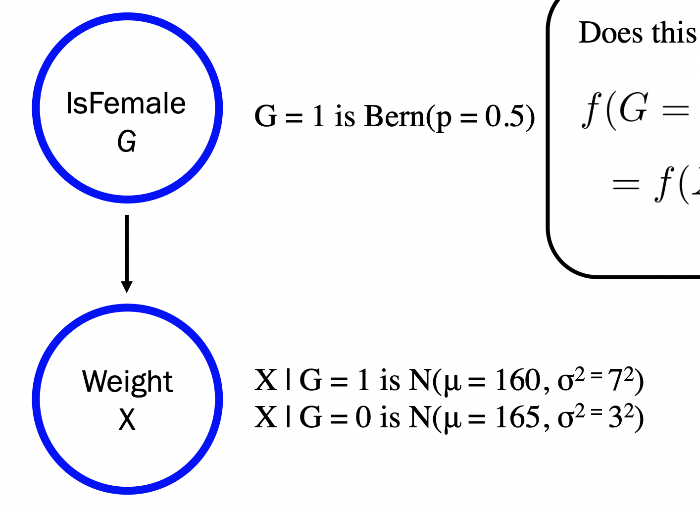
Much more efficient and computationally tractable to reason about conditionallity (i.e. answer questions like “What is \(P(G=1 \mid X=163)\)?”) than the entire joint!
We will explore this graphical idea in the next lecture. Back to Bayes’!
Calculating normalization constant:
- Problem solving tip: you might be given two Bayes’ with continious RV’s and want to find “likelihood that this is greater than that”. Before deriving the actual formula, you can cancel out the normalizing constant because you are dividing a fraction by a fraction.
- Other times, you’ll actually need to derive the denominator using law of total probability.
- Also you can get denom. by figuring out what value sums to 1 for all of the possible posteriors by the third axiom.