Lecture 12: Inference part I

We can then apply Bayes’ theorem to a multinomial. See Federalist papers example.

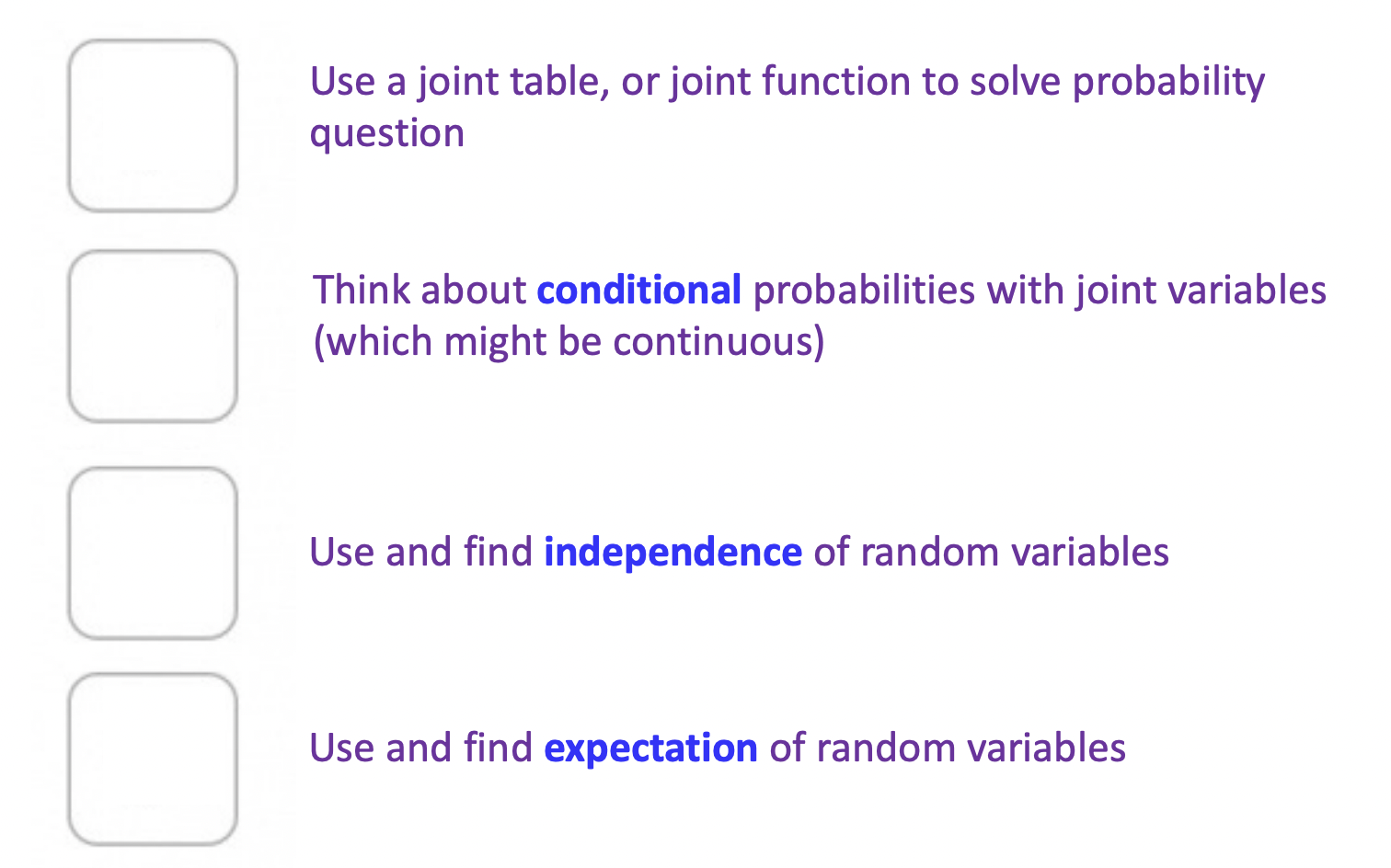
What you need to know for this unit:

|500

Inference

Definition (inference): An updated belief about a random variable (or multiple) based on conditional knowledge regarding another random variable (or multiple) in a probabilistic model. TLDR: conditional probability with random variables.

This makes sense. We want to use that probabilistic graphical model to infer different things regarding conditionalities.

• Example: say you have a joint table with dorm type on one axis and year in uni on the other axis. Conditional probability would be like “what is the probability that you have a single given that you are a senior”. It is important to note the difference between joint and conditional probability. One is \(P(X=x, Y=x)\) and the other is \(P(X=x | Y=y)\)… very different equations! In the last example, joint would be “what is the probability that you have a single and that you are a senior”. Marginal is then a random variable (not a probability!): \(P(X=x \mid Y=2)\).

Bayes’ variants

At its heart, conditional probability with multiple random variables heavily relies on Bayes’ theorem (because we’d often be given or be able to derive the reverse conditional). There are many Bayes’ variants when it comes to working with two random variables (because some RVs are continious whereas others are discrete). Remember that Bayes’ theorem and probabiliteis in general works with events (i.e. the RV taking on a value) not just random variables (which are objects) by themselves.

I. Discrete/discrete Bayes’

Practically the og Bayes’: two discrete random variables taking on a specific value where one depends on the other.

Discrete/discrete Bayes’: Let \(M\) and \(N\) be discrete random variables. Then, by Bayes’ theorem: \[P(M=m \mid N=n)=\frac{P(N=n \mid M=m) P(M=m)}{P(N=n)}.\] Law of total probability way: \[P(M=m \mid N=n)=\frac{P(N=n \mid M=m) P(M=m)}{P(N=n \mid M=m) P(M=m) + P(N=n \mid M=m^{C}) P(M=m^{C})}.\]

We are referring to the probability of \(M\) taking on a specific value (event) given that \(N\) has already taken on a value. Example:

\[P(M=2 \mid N=3)=\frac{P(N=3 \mid M=2) P(M=2)}{P(N=3)}.\]

Often, we’ll use the shorthand notation:

\[P(m \mid n)=\frac{P(n \mid m) P(m)}{P(n)}.\]

Bayes’ theorem with discrete RV’s is easy: it is just a table with a bunch of lookups. The real complexity arises when you have a continious random variable in the mix because now you are dealing with densities instead of probabilities. We will explore that in the next lecture.