Lecture 11 - Probablistic models
- Inverse CDF can be used for drawing samples from a distribution.
- Poisson and normal approximations. Use normal when \(p\) and \(n\) fall in certain range and Poisson for different values of \(n\) and \(p\).
- Proportional: self-explanatory: use this symbol when you want to talk about a number being proportional to something (i.e. scalar multiple for some constant).
Relative probability
- We know that we cannot measure the exact probability for a CRV because we work with densities not probabilities. However, there is a neat property: if we are asked about the ratio/proportion of two probabilities that are continious, we can use PDF’s directly without integrating.
- Example scenario: “How much more likely are you to complete in 10 hours than in 5?”. Let \(X \sim N\left(\mu=10, \sigma^{2}=2\right)\).
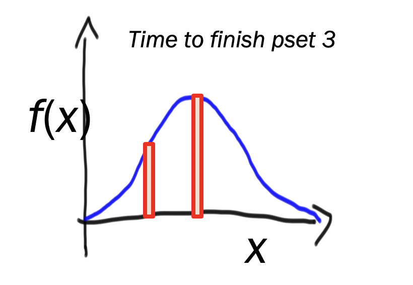 Probability density is point on curve whereas probability is area. How to get area under curve? We need a bit of width to make a rectangle. We call this width value \(\epsilon\) which is infinitestimly small. So we have: \[\begin{aligned} \frac{P(X=10)}{P(X=5)} &=\frac{\varepsilon f(X=10)}{\varepsilon f(X=5)} \\ &=\frac{f(X=10)}{f(X=5)} \end{aligned}.\] And bam. Just like that we have a simple function calculation!
Discrete probabilistic models
- We know how to model real world phenomonom using single random variables. But the real power is when we join them together. We can model complex networks from real life and how these nodes of the network interact (e.g. how they depend on each other… conditional probability!) in a probabilistic framework. e.g.
 .
. - Example: webmd. Takes in symptoms and gives possible illnesses. Can think about modelling each symptom/disease a random variable and seeing how they interact jointly to make inferred predictions.
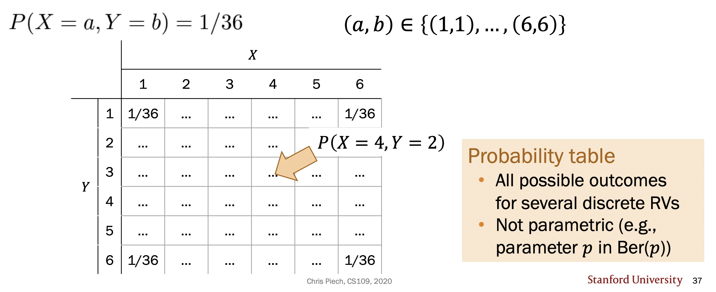
- In the single variable case, we defined a PMF which was able to give us the probability of the RV taking on a specific value (i.e. an event). In joint distributions, we care about both of them taking on particular values (“and”). JPMF gives you complete information for distribution. \[P(X=a, Y=b)\] means “what is the probability that \(X=a\) and \(Y=b\)?”.
- We often represent joint distributions using “tables”:
- Theorem: Let \(X\) and \(Y\) be jointly distributed random variables. Then, by the Kolmogorov axioms: \[\sum_{x \in X} \sum_{y \in Y} P(x, y)=1\]
- Assignments in a joint distribution are mutually exclusive (i.e. \((X=x)\) must be distinct for different values of \(x\)).
- Syntax shortcut: \(P(x, y) = P(X=x, Y=y)\).
- Marganilization: we often want to know what the probability of \(X\) taking on some value is given that we are holding \(Y\) as constant. To do this, we loop over all the possible probabilities of \(X\) taking on some value with the corresponding constant \(y\). This is called marganilization.
- Limitations of the joint: a key realization that we had is that specifying the joint gives us everything we can possibly want to know about the joint model’s RV’s. So why do we have five more lectures on this concept. What is more to it? The problem is, as you add more random variables, the joint continues to increase in size and becomes too large to do anything useful computationally. So we must develop clever “tricks” for working with large joints (i.e conditional probabiliy).
- Think about it like this: a 2 RV joint distribution can be represented by a grid (2-dimensional). 3 RV system now requires a cube (an extra dimension). As we grow our model (as we often will do the real world), we will need insane number of dimensions for our (hyper)-“table”.
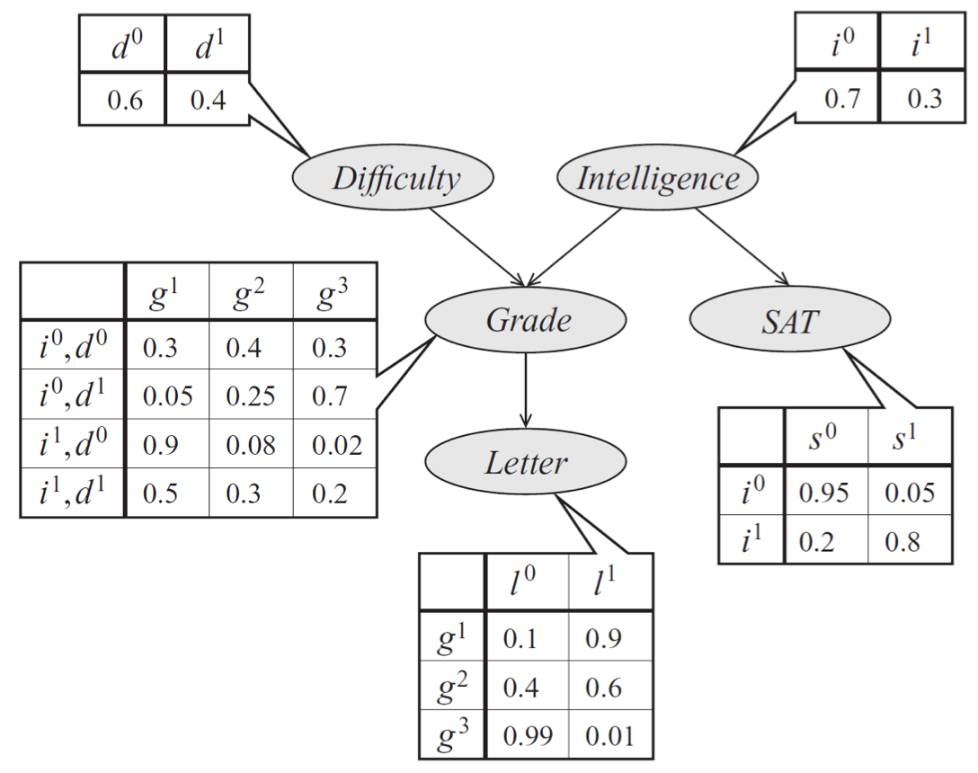
- Example: Let us say we have a system of 10 RV’s each of which can take on 5 different values. We have \(5^10\) different combinations. With only 10 RV’s! Staggering. We need to introduce some nice theory to work with this stuff more usefully (hint hint: conditional probability). That is, we need to introduce probabilisitc graphical models where the nodes represent random variables and the edges denote conditional dependence. Now we’d have one giant probabilistic system. And using these models we could start to infer different things about the system without needed the computationally intractable full joint.
Multinomial
Our first “probabilistic model” (i.e. it is parametric) is the multinomial.
- We defined the binomial based on number of heads in consecutive coin flips. We let \(X\) be a binomial random variable which represented number of heads. We could have alsod defined \(Y\) to be number of tails.
- In dice rolling, the options aren’t binary. So instead, we define a random variable for each side: how many times does a 3 appear–let this be a random variable and so on.
- So intead of there being 2 possible outcomes like in binomial, we have \(n\) different number of outcomes.
- Example:
- So now we can answer questions relating to dice roll type experiments using the PDF of a multinomial.
- At its root, a multinomial is a counting idea (the multinomial coefficient). A good application is language: count number of words etc. Lots of ties to conditional probability (inference!) which is what we will learn about next.
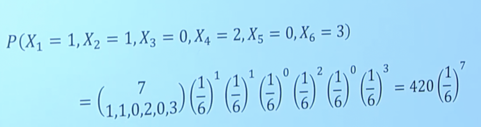
Definition (Multinomial): let’s perform \(n\) independent trials of an experiment where each trial results in one of \(m\) outcomes, with respective probabilities: \(p_{1}, p_{2}, \ldots, p_{m}\) (constrained so that \(\sum_{i} p_{i}=1\) ). An example of this would be a dice roll. Let \(n=1\) (one dice roll) and \(m\) is going to be \(=6\) because there are \(6\) possible outcomes. Now, a multinomial distribution is a closed form function that answers the question: What is the probability that there are \(c_{i}\) trials with outcome \(i\)? Mathematically: \[P\left(X_{1}=c_{1}, X_{2}=c_{2}, \ldots, X_{m}=c_{m}\right)=\left(\begin{array}{c}n \\ c_{1}, c_{2}, \ldots, c_{m}\end{array}\right) \cdot p_{1}^{c_{1}} \cdot p_{2}^{c_{2}} \ldots p_{m}^{c_{m}}. \] That is, you can imagine assigning a random variable to each of the \(m\) outcomes (e.g. dice side six) that happens with probability \(p_i\). But we have \(m\) different random variables so we have a joitn distribution. And we care about all of them satisfying certain equalities. Example: Let us roll a six-sided \(m=6\) dice \(n=10\) times. We can specify a random variable \(X_i\) for each of the \(m\) outcomes (side that the dice lands on) that represents the number of times in \(n\) trials that we will see that outcome (e.g. \(X_6\) might represent “how many 6’s appear in \(10\) dice rolls?”“). Now we are interested in e.g. \(X_1\) taking on the constant \(2\) and maybe \(X_4\) taking on the constant \(5\) and so on. This is a joint probabiliy distribution! In the case of dice rolls, each RV has equal parameter \(p\) but that won’t be the case always as we will see in the document example (which leads into conditional probability for multiple random variables).
We can then apply Bayes’ theorem to a multinomial. See Federalist papers example.